¶ Digital Twin of a Human Cell
Members: Sahasra BobbalaUG, Nikhil GulveUG, Arnav KumarUG, Sahana MandayamHS, Kashvi ShahUG Faculty: Wade Trappe, Ivan Seskar, Jenny Shane
¶ Our Goal
This project is an interactive, educational 3D simulation of a living cell built to help biology students see how a cell actually works. Instead of treating the cell as a single well-mixed bag of chemicals, it divides the cell and its surroundings into a 3D grid of tiny voxels, each tracking local concentrations of substances like oxygen, glucose, and ATP. Using a reaction–diffusion model (Fick's law for movement, Michaelis–Menten kinetics for reactions), substances spread realistically between neighboring voxels while organelles such as mitochondria carry out processes like aerobic respiration and fermentation. The heavy computation runs on an H100 GPU and streams live to a browser, where students can rotate the cell, inspect color-coded organelles, introduce oxygen or glucose into the environment, and watch them diffuse across the membrane and get converted into energy in real time — all designed as a teaching tool to make invisible cellular processes visible and explorable.
¶ Weekly Progress
WEEK 1 (05/25-05/28)
Week 1 Presentation
- Installed the needed softwares
- Configured SSH Keys
- Set up our Wiki
- Set up GitHub
WEEK 2 (06/01-06/04)
Week 2 Presentation
- Changed our direction towards the project
- Researched and modelled a human cell
- Researched digital cloning for human cells
- Built a model to visualize basic parameters
WEEK 3 (06/08-06/11)
Week 3 Presentation
- Researched aerobic and anaerobic respiration, and measuring unit
- Broke down aerobic and anaerobic respiration into code
- Increase the accuracy of the model for the aerobic and anaerobic respiration
WEEK 4 (06/15-06/18)
Week 4 Presentation
- Stepped back to rethink how we use LLMs in our workflow
- Built and refined the cell simulation demo
- Worked through how to handle time inside the cell
To redine our AI use,
- Context Injection
- Stores our knowledge base (Edison lab research, papers, docs) as searchable sources, then retrieves only the relevant ones at query time to ground each answer. Automated and scales as our docs grow.
For our discrete time problem,
- A real cell runs continuously — a simulation can't, so we step time in fixed intervals: t(x) = t(x−1) + Δ
WEEK 5 (06/22-06/25)
Week 5 Presentation
- Dug into how the back end and front end actually fit together.
- Began assembling the formulas that drive the simulation.
- Started untangling which processes run in sequence vs. at once.
The essential bio101 processes we want to focus on,
- Membrane transport
- Glycolysis
- Oxidative phosphorylation
- Fermentation fallback
- ATP budget
- Transcription & translation
Also focused on which formulas are strictly sequential, and which should run simultaneously and their difference.
WEEK 6 (06/29-07/02)
Week 6 Presentation
-
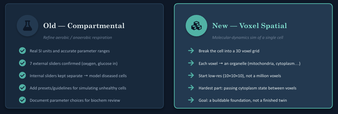
Split the project into two teams; refine the old compartmental model, build the new spatial one.
-
Worked out the GPU server + VR streaming split for both models.
-
Got access to the H100 GPUs that make the spatial model feasible.
-
Old Model vs New Model:
WEEK 7 (07/06-07/09)
Week 7 Presentation
- Moved the compartmental backend onto the WinLab servers.
- Started building toward many instances running on the H100.
- Grew the diffusion matrix and hosted it on the P100 server.
- For the old model, exposed temporal granularity controls directly to the frontend.
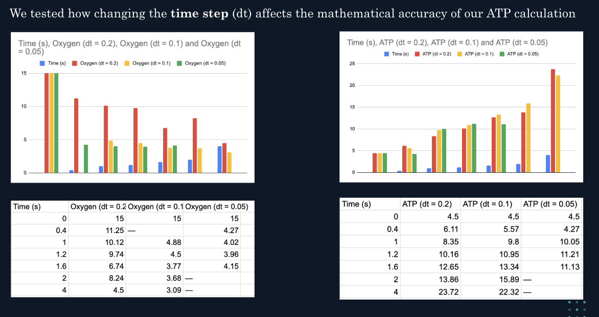
- Users can modify the numeric integration interval (dt) from 0.20s down to 0.01s
- A smaller dt prevents the ODE solver from breaking down or producing negative concentrations during hyper-metabolic shifts.
- Hosted the site on WINLAB servers, to make it publically accessable via the WINLAB WiFi
WEEK 8 (07/13-07/16)
Week 8 Presentation
- The new spatial model now runs on the P100 at roughly 800,000 voxels.
- Installed CUDA; the GPU compute stack is in place — diffusion now runs in parallel.
- Decreased the time interval on the old model, resolving the artifacts.
- Env variables & distance defined
- Met with chemical engineers to help us with our graphs for the old model
WEEK 9 (07/20-07/23)
Week 9 Presentation
- Finished the old model; Documented, wrapped as a final version, packaged as a .exe and hosted.
- H100; NVIDIA drivers + toolkit installed, CUDA running, model built with CuPy.
- New model broken into a clean frontend and backend separation.
- Teams merging to work towards the new model
WEEK 10 (07/27-07/30)
Final Presentation Practice Run
- Our Project
Interactive digital twin of a human cell for Bio 101 Two builds in parallel: compartmental whole-cell model + GPU-accelerated spatial voxel model Python simulation backend + live web interface
3D Spatial Model
- Spatial Model Overview, based on the Fick's 2nd Law, ∂C/∂t = D∇2C + R(C) - substances spread from crowded areas to emptier ones
- Stability requires α = D·dt/dx² ≤ 1/6, enforced so the simulation can't blow up to NaN
- Tiny 3D cubes, like pixels but in 3D - each organelle gets its own voxel type and color
- Scaling roadmap: 4³ start → 800,000 voxels on the P100 → ~8 million goal on the H100
- For the spatial diffusion, Builds the cell in 3D and tracks how things spread through it, not just totals
- Backend runs on GPU (CuPy); frontend streams over WebSocket and renders with Three.js
Compartmental Model

- Whole cell as a broken down, architectural tree, think of it as objects within a class.
- Input sliders with 6 parameters, Glucose, O₂, and Nutrients sliders to change various processes, Infection, DNA damage, and Toxin events inject a pathological state that cascades across agents
- Based on Michaelis-Menten Kinetics rate = Vmax·[S] / (Km + [S]) e.g. mitochondrial ATP rises with glucose × O₂, but flips to anaerobic below the O₂ threshold (Pasteur effect)