¶ Project: Channel Measurement Campaign for Data Analytics
Project Members
Derek Ling
Tyler Thomassen
Srishti Hazra
Advisors
Ivan Seskar
¶ Project Overview
Goal: Create a labeled, machine-readable channel model dataset spanning as many signal types, frequencies, and power levels as possible. The ultimate objective is to replace traditional SDR algorithms (which rely on hand-crafted DSP and idealized channel models) with AI models trained on real-world RF data. The dataset serves as the training corpus for neural networks to learn channel behavior from ground truth, improving generalization over rigid mathematical models.
Approach: We utilize the COSMOS/ORBIT testbed to perform controlled wireless experiments. We capture raw IQ data using USRP nodes (specifically Sandbox 7 and the wider grid) and integrate the SigMF standard for metadata management. Our pipeline evolves from basic GNU Radio flowcharts to automated Python-based scripts that handle data capture, post-processing (SNR, BER, CFO), and final ingestion into a vector database for search and retrieval.
¶ Weekly Progress
Week 1: Onboarding and Environment Setup https://docs.google.com/presentation/d/1D2OUZyUC9shGFYABVgAm0Ezi35X3_Y2BJ9HrsjzabZ0/edit?slide=id.g3a8cc5f8fa6_0_3684#slide=id.g3a8cc5f8fa6_0_3684
During the first week, we focused on onboarding and familiarizing ourselves with the project's overarching goals and the technical environment. We introduced ourselves and the project's mission to replace rigid SDR algorithms with AI trained on a comprehensive RF dataset. The core objective was to deploy an SDR platform across the COSMOS/ORBIT testbeds to capture labeled IQ data across varied conditions (frequency, environment, antenna config).
To achieve this, we focused on three main learning areas: understanding the ORBIT testbed workflow, including the use of OMF commands and secure SSH access to the console and nodes; practicing fundamental Linux commands for directory navigation and file management; and learning the basics of Software Defined Radio (SDR), specifically the representation of radio signals using complex IQ samples (In-phase and Quadrature components) to describe amplitude and phase.
Week 2: GNU Radio Fundamentals and Signal Capture https://docs.google.com/presentation/d/1gbTmQ23vhYKIGh1HkP9oVu8cmr-fby0TV4yflofkmjw/edit?slide=id.g3e8420d5dcb_0_0#slide=id.g3e8420d5dcb_0_0
In the second week, we moved from theoretical understanding to practical implementation by mastering GNU Radio and the USRP hardware. We created flowcharts for transmitting and receiving controlled known reference/pilot signals. We successfully executed experiments using the USRP2 in Sandbox 7 (SB7) by working through COSMOS tutorials and running experiments to transmit and receive signals on the USRP.
We delved into the specifics of signal generation (where a signal source generates digital IQ samples, which are sent via UHD to the USRP to be converted to RF) and signal reception (where the USRP captures RF, converts it to IQ samples, and sends them to GNU Radio for visualization via FFT). We also increased our knowledge of channel modeling concepts, including scattering and pathloss. A significant challenge this week was overcoming the complexity of managing multiple terminals, GNU Radio versions, and mismatched configurations to successfully bridge the transmitter and receiver.
Week 3: Recording IQ Data and Extracting Measurements https://docs.google.com/presentation/d/1TrLuYk5gkFJBUm3n6kkDYxl7RiLisnLPJMwy_l_tLcs/edit?slide=id.g3eafc11caab_5_1218#slide=id.g3eafc11caab_5_1218
Week 3 marked our transition into running our first controlled experiments and establishing a foundational pipeline for data processing. We extended our GNU Radio receiver flowgraph by adding a file sink, allowing us to permanently store raw IQ samples from each experiment as .dat files instead of just visualizing them in real-time.
To make sense of this raw data, we created a Python analysis script (analyze_iq.py). This script reads the captured IQ samples and computes key channel metrics, including Received Power (dB), Signal-to-Noise Ratio (SNR), and Channel Gain. The output of this script is a structured CSV dataset, which allows us to easily visualize and analyze how the channel behaves as we change parameters (such as gain).
Week 4: Metadata Standards and Why We Need SigMF https://docs.google.com/presentation/d/1tDQMOg7H909ldch0CIk0LsSEnEFlRjs-REqG1oG5sPg/edit?slide=id.g3edb8dec2a0_3_3429#slide=id.g3edb8dec2a0_3_3429
As we scaled our experiments, we realized that raw IQ samples alone are insufficient. A file containing only IQ samples does not tell us which node transmitted, which node received, the center frequency, sample rate, or gain used. Without this metadata, large datasets become difficult to organize and analyze, and they are largely useless for training AI models.
To solve this, we integrated SigMF (Signal Metadata Format) into our workflow. SigMF is an open standard that pairs raw IQ data (.sigmf-data) with a structured JSON metadata file (.sigmf-meta). This ensures that every dataset is fully self-describing, interoperable across different SDR software, and machine-readable. We mapped out how post-process metadata—like SNR, BER, and CFO—gets computed and appended back into the SigMF annotations array.
Week 5: OFDM Sweeps and Moving to Python Automation https://docs.google.com/presentation/d/1lpjBrfYQ1ggUGAkSLW-HlonT9EnbAQA3H9NrcUqtR1Q/edit?slide=id.g3ef31e784c4_1_34#slide=id.g3ef31e784c4_1_34
This week, we made a critical infrastructure shift. We identified that the old workflow (dragging and dropping GNU Radio Companion blocks and manually changing parameters for each individual experiment) was not scalable, hard to reproduce, and lacked automation.
We replaced the GRC manual workflow with a modular Python script architecture. We developed tx.py (transmitter), rx.py (receiver), run_experiments.py (the automation engine), and experiment_config.py (centralized parameter control). We tested this new framework by running OFDM sweeps across multiple TX gain levels (0dB, 5dB, 10dB, 15dB). Additionally, we designed a robust Day/Night automated pipeline: experiments capture data during the day, and an automated script pulls files, post-processes them (calculating SNR, BER, CFO, Frame Count), writes the results back into the SigMF metadata, and ingests the final labeled dataset into a database overnight.
Week 6: Constructing the BPSK Pipeline and Establishing a Baseline https://docs.google.com/presentation/d/1RKwz1tOsXdjRYXWVyPbLLx5IGnNLiHog-L1HhO_lhOE/edit?slide=id.g3ef31e784c4_1_0#slide=id.g3ef31e784c4_1_0
In Week 6, we focused on constructing a dedicated BPSK pipeline to establish a single-frequency, single-power baseline. We generated a reference bit file, transmitted the signal over-the-air using our USRP B210, and captured the unprocessed IQ samples. We established a strict three-file output per experiment: the raw IQ capture file, a metadata file (with TX/RX node IDs and frequency), and the random bit file used for the transmission.
This structure allows us to run a "Classical Demod" (using a GNU Radio BPSK receiver) alongside an "AI Model Demod" (which takes the IQ data and attempts to recover the bits). By comparing the demodulated bits to the reference bit file, we can compute a definitive BER for both methods. The post-processing pipeline was also refined to focus exclusively on calculating and comparing BER and SNR above all else.
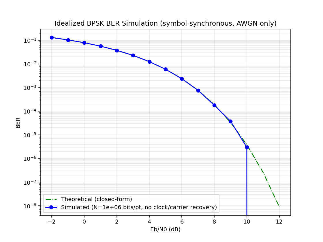 Figure: Theoretical BPSK bit-error-rate curve over an AWGN channel, used as the baseline reference curve against which the Week 6 classical and AI demod BER results are compared.
Week 7: Phase Lock Issues, Differential Demodulation, and BER Analysis https://docs.google.com/presentation/d/1YiL3jdu_WLRPYNsU5Ttiii2DgDGMwRWYbn2-i-q82lc/edit?slide=id.g3f434360ac7_2_202#slide=id.g3f434360ac7_2_202
Deploying our BPSK pipeline onto the wider grid revealed a critical issue: the Costas Loop used for coherent demodulation was failing to lock onto the carrier phase. While the code worked perfectly on Sandbox 7 nodes, experiments on the wider grid produced a "ring" scatter plot, indicating amplitude collapse and a failure to lock the absolute phase. Raw IQ and power spectrum plots showed the signal was getting through clearly, so the issue was in the demodulation stage.
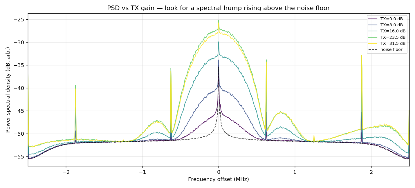 Figure: Raw IQ and power spectrum overlay confirming the signal was reaching the receiver cleanly, isolating the fault to the demodulation stage rather than the RF link.
We solved the phase lock problem by switching to differential detection (comparing the phase of adjacent symbols instead of trying to lock to an absolute phase). This immediately produced tight clusters in the scatter plot. We ran an extensive 11-trial matrix across multiple frequencies (900 MHz, 3.5 GHz) and distances (~1m to ~9.9m). While close-range and differential schemes achieved perfect 0 BER, long-distance coherent detection hovered around 50% BER (random guessing). Switching to differential detection at long distances produced the expected "waterfall" curve, drastically reducing BER.
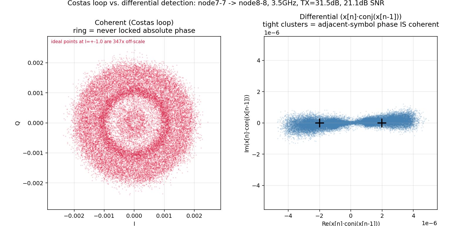 Figure: Comparison of the Costas-loop coherent demodulator's "ring" scatter artifact on the wider grid against the tight clusters recovered after switching to differential detection.
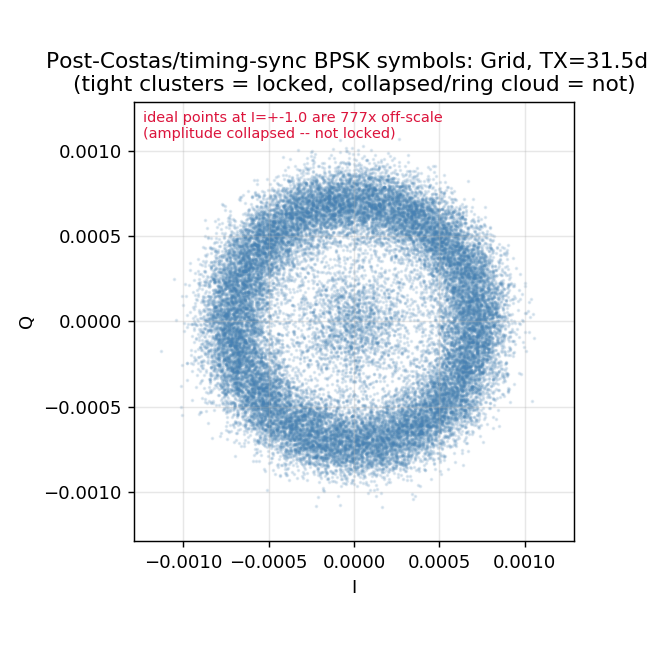 Figure: Recovered symbol constellations across the 11-trial matrix spanning 900 MHz and 3.5 GHz at distances from ~1m to ~9.9m.
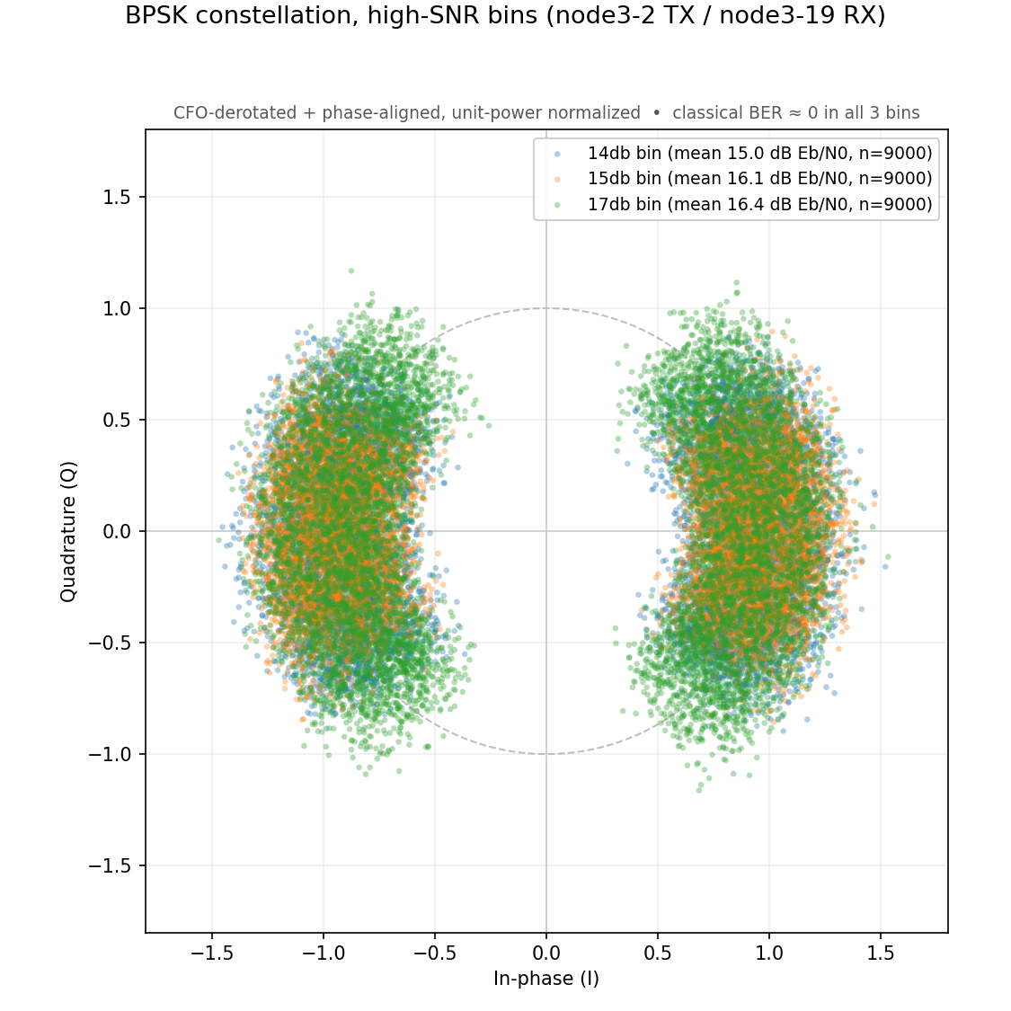 Figure: BPSK constellation at high-SNR bins (node3-2 TX / node3-19 RX) after switching to differential detection - tight, well-separated clusters with classical BER approx. 0.
Week 8: Pilot Resync, Returning to Coherent, Ansible Automation https://docs.google.com/presentation/d/1JVtS5W1zaFeiYd8gJFF36prvAaIMGwqfbc0jhrC37l8/edit?slide=id.g3f53dd1de11_0_0#slide=id.g3f53dd1de11_0_0
After the previous week's detour into non-coherent recovery on the grid, we made the decision to return to coherent demodulation. We solved the cycle-slip issue by building a pilot-anchored resynchronization scorer. By correlating against a known pilot pattern that repeats between data blocks, the scorer re-derives alignment from scratch after a slip, containing the damage to a single block. The found/missed pilots give us a free per-block lock map, so BER is only measured where the receiver was genuinely locked.
We validated this from simulation through to over-the-air. After confirming a clean waterfall curve in a GNU Radio BPSK simulation and an SB7 pilot-resync simulation, we ran it OTA on corner radios 20 meters apart, linked through an ultra-precise GPS master clock, and achieved a BER within 3 dB of our benchmark. Phase-tracking analysis showed one trial locked perfectly for 0% BER, another tracked cleanly for the first half before losing lock, and a third never locked. Isolating these hardware synchronization issues means the bit errors we measure come strictly from the wireless channel. On the infrastructure side, we began adopting Ansible to eliminate manually SCP-ing scripts to each node, automatically kill stuck jobs, and make experiments modular.
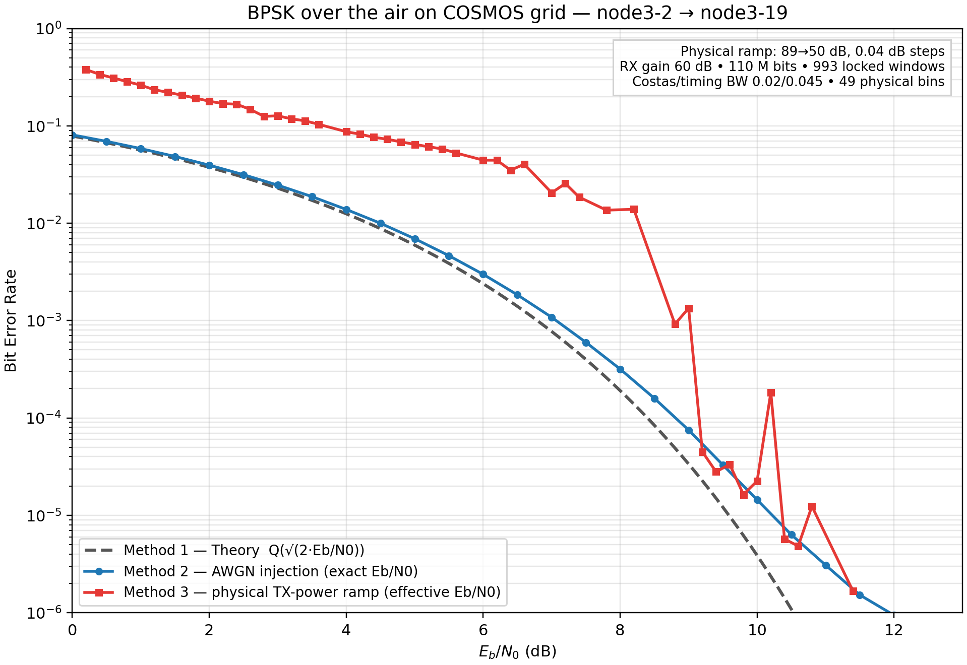 Figure: BPSK over-the-air BER on the COSMOS grid (node3-2 to node3-19), comparing theory, AWGN-injection emulation, and the physical TX-power ramp - the OTA results track the benchmark curve closely, confirming the pilot-resync approach.
Week 9: Baseline into Ground Truth and Choosing an ML Architecture https://docs.google.com/presentation/d/11WWKf0YAbOD0jtPfQvTNv59Obdp8Bp4QpWzxO8_Ve5E/edit?slide=id.g3f434360ac7_2_202#slide=id.g3f434360ac7_2_202
We rebuilt the reciever so the loops now lock once and stay locked for the whole run, gain ramps continuously while that lock holds, and an FLL front-end pulls in the coarse frequency offset that was causing slips. It also correlates against long PN sequences for robust alignment and takes longer captures at low SNR, where more data is needed to get a clean BER. After ~6 hours of trials to smooth the low-BER region, we reached a curve within 3 dB of benchmark, which we now treat as ground truth.
We validated repeatability with physical TX-power ramps over the air. Running 49 independent trials with identical settings showed genuine OTA variability while most followed the same waterfall trend; averaging BER across matching Eb/N0 intervals revealed the underlying physical waterfall and a more reliable performance estimate. For the ML, we chose 1D-ResNet as our starting point for supervised demodulation: IQ in as two real channels, using known TX bits as labels, and BER as the metric.
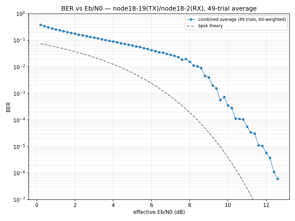 Figure: Combined 49-trial average BER vs effective Eb/N0 (node18-19 TX / node18-2 RX). This averaged curve is the ground-truth benchmark used for later ML comparisons.
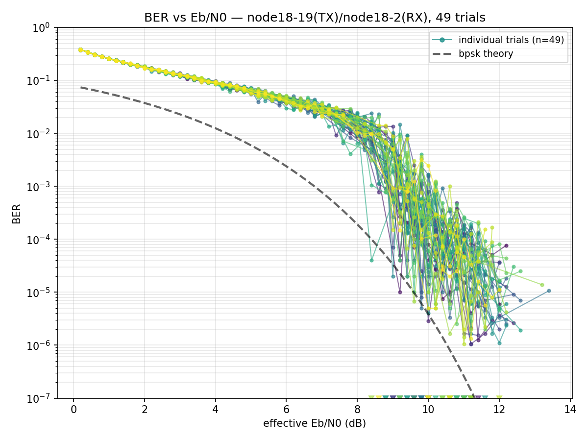 Figure: BER vs effective Eb/N0 for each of the 49 individual trials, showing genuine OTA variability around the shared waterfall trend before averaging.
Week 10: ML Architecture Results and the Low-SNR Challenge https://docs.google.com/presentation/d/16WELYmjNMN2_82BmSHemGQXC7Rp04kOuaEqVAtVBXWI/edit?slide=id.g3f5eab7910f_2_83#slide=id.g3f5eab7910f_2_83
This week we produced our first real machine-learning results by putting the architecture from Week 9 to the test. With the continuously-locked FLL baseline serving as ground truth, we trained three architectures on the same high-SNR OTA data: ResNet1D, GRU1D, and TCN1D. ResNet1D achieved the lowest BER (~10⁻³) but was unstable late in training, spiking sharply near the end of the run. TCN1D converged to nearly the same accuracy roughly 5× faster than ResNet, making it the better choice when we need to iterate quickly, while ResNet remains the pick for the best final number. GRU1D was both the slowest and the least accurate, and is a poor fit for this task.
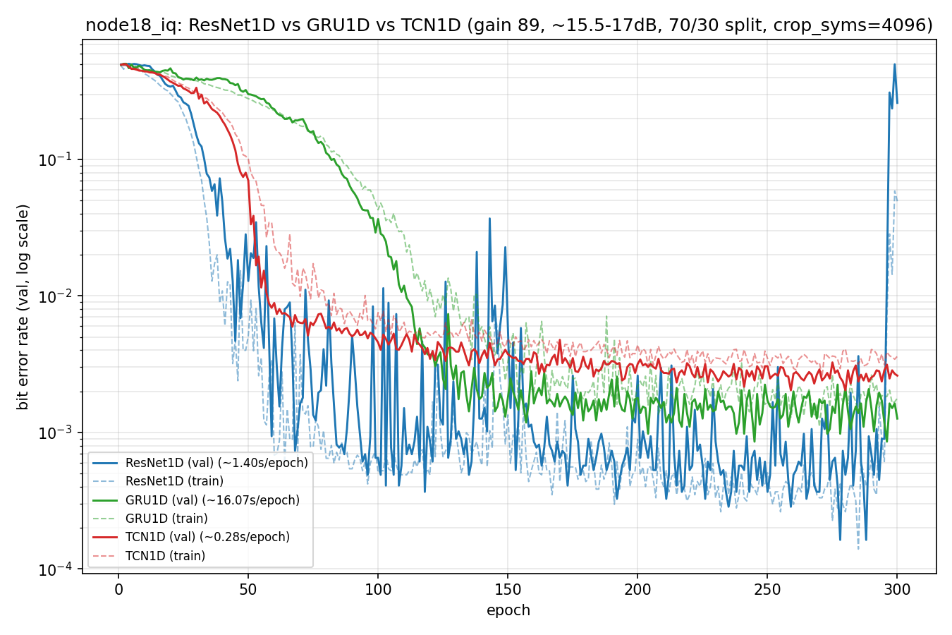 Figure: Validation bit error rate vs training epoch for ResNet1D, GRU1D, and TCN1D on node18 IQ data. ResNet1D reaches the lowest BER but destabilizes late in training, while TCN1D converges to near-equal accuracy far faster.
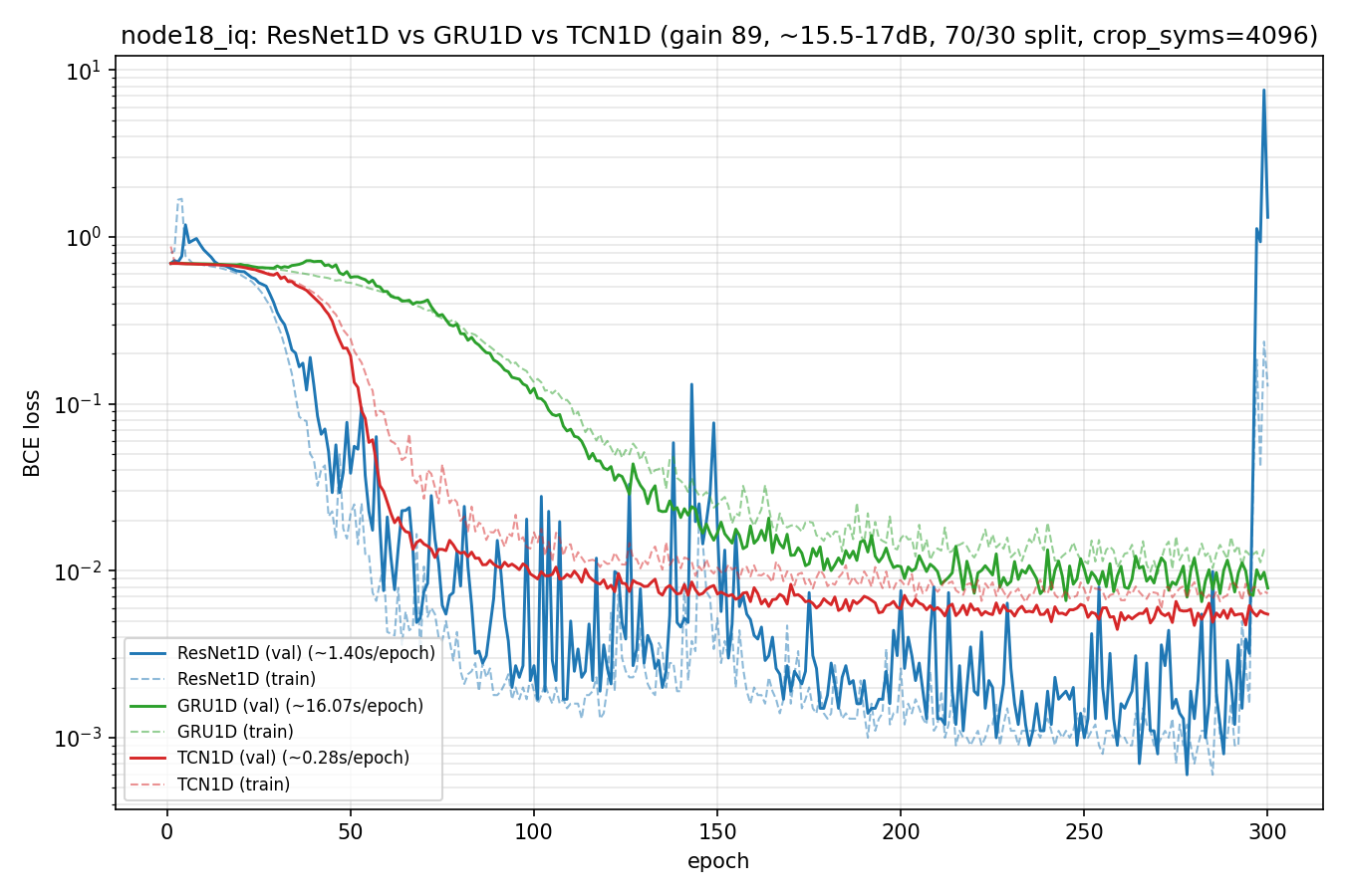 Figure: Validation and training BCE loss vs epoch for the same three architectures, mirroring the BER trends above.
We trained across eight SNR bins from 3–17 dB and tested on held-out captures, both ResNet and TCN reach ~10⁻³ at high SNR and are competitive with classical DSP at the top end, but below ~12 dB all models plateau near 50%, and are not yet generalizing to low-SNR conditions. We still need more captures and more channel diversity to address this issue.
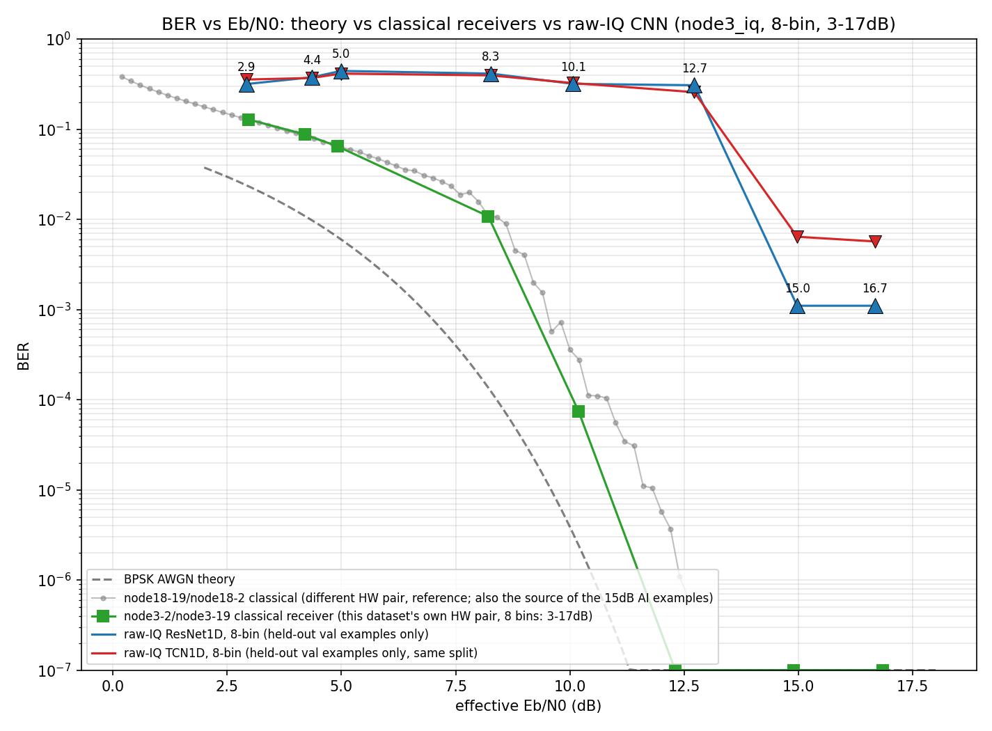 Figure: BER vs effective Eb/N0 comparing theory, classical receivers, and raw-IQ ResNet1D/TCN1D across 8 SNR bins (3-17 dB). The AI models match classical performance at high SNR but plateau near 50% BER below ~12 dB.
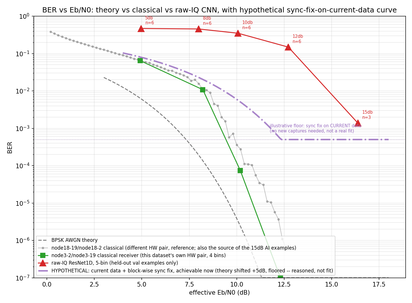 Figure: Illustrative projection of the low-SNR BER floor achievable with a block-wise synchronization fix applied to the current dataset (not a fit to real data), motivating our planned next steps.