¶ IoT Device Identification Against Shaped Traffic
Member: Praneeth Damarla
Faculty Advisor: Prof. Anand Sarwate
¶ Project Overview
As the number of Internet of Things (IoT) devices in households has increased year by year, there have been significant privacy risks, including the risk of these devices leaking daily user routines to attackers outside your home network.
This is done simply by observing the packet timing and sizes in the headers of encrypted network traffic sent from your home router.
With only this information, these attackers can accurately identify specific IoT devices in your household and infer your activities.
E.g.:
- Amazon Echo: Knows when you are conversing with the voice assistant
- Smart Camera: Knows when you are in the frame of the camera
- Sleep Sensor: Knows when you are resting
Prior work has shown that traffic shaping can obfuscate network traffic by perturbing packet size and timing, preserving privacy.
For the scope of this project, we focus on the device identification step in this threat model, rather than on downstream activity inference, due to dataset restrictions.
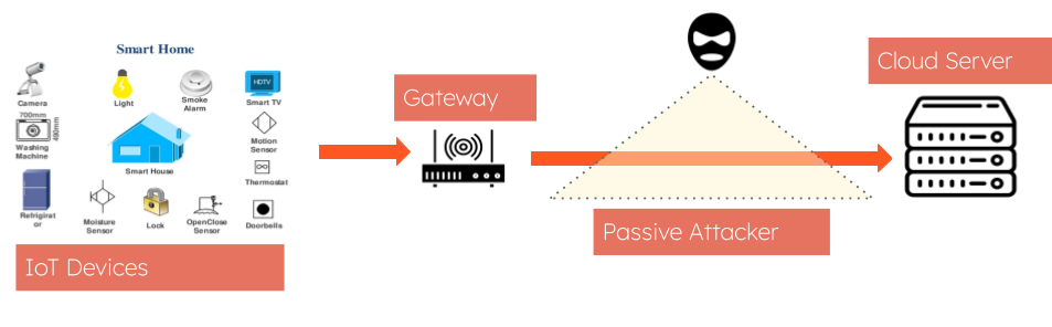
The figure below illustrates where the passive attacker sits within a household's network path.
Goals of Project:
- Clean and prepare a dataset of network traffic from several IoT devices
- Develop a reasonably accurate device fingerprinting model with machine learning trained on the above dataset
- Evaluate the effectiveness of multiple traffic shapers against the fingerprinting model
¶ Weekly Progress
¶ Week 1: Project Introduction (Presentation)
- Oriented myself to the project and field of machine learning for network privacy
- Performed an initial literature review on machine learning-based attack models
¶ Week 2: Dataset and Tech Stack (Presentation)
- Found primary dataset with 20 days of captured network traffic for ~30 IoT Devices
- Preprocessed dataset from PCAP to CSV with TShark, preserving WAN-bound traffic via TCP or UDP
- Developed an understanding of various machine learning classifiers, including CNN, LSTM, and Random Forest
¶ Week 3: Literature Review (Presentation)
This week, the literature review was narrowed to a single paper that includes source code for fingerprinting models and traffic shapers. Below is a link to the paper:
Most recent papers found during the literature review primarily lacked publicly available source code and/or did not focus on attackers who only eavesdropped.
The paper details two types of device fingerprinting models based on methods for handling time-series data, since network traffic is intrinsically a time series.
The rest of the week was spent analyzing the source code to identify the main features, ranging from packet size and timing to be fed into the machine learning models.
¶ Week 4: Device Fingerprinting Models (Presentation)
For all models, the data is split into individual CSV files, each containing network traffic for a specific device-day combination. For example, AmazonEcho_September_23_2016.csv would be one such combination.
Below are detailed descriptions of the two fingerprinting models that were analyzed during the previous week:
-
Sequential Model (CNN, LSTM, GRU, MLP): This model takes an n second window/sample from your data and then samples this window by m seconds, where n and m are manually tunable parameters. This creates a total of n x m time slots within the window, where, in each slot, the total packet size sent from the router and the total packet size sent to the router from all packets in that slot are the two features tracked. This captures the distribution of traffic being sent and received every n seconds. Additionally, each window is not exactly n seconds long, as n represents the minimum wait before creating a new window. A new window is created once the next packet after n seconds has been sent. The last feature engineered is the time of silence between windows, which captures the "chattiness" of the device. Let D be the length of the input vector (this is also the number of windows). Then, once processed, the dataset becomes a tensor of size D x (n x m) x 2, along with a separate column vector containing the silence periods between windows. The machine learning architectures chosen for this model are a 1D CNN, LSTM, GRU, and MLP. CNN and LSTM were chosen as the primary subset for investigation. The pipeline begins with the data tensor passing through the feature-learning layers of the CNN and LSTM, including the CNN's 1D convolution layers and the LSTM unit. Once the data has passed through these layers, the silence vector is concatenated with the flattened data vector. This concatenated data vector is then sent through the final MLP layers to obtain a prediction.
-
Aggregate Model (Random Forest): This model takes p minute windows/samples from your data and aggregates statistics for all packets sent and received within the window based on the total packet size. The statistics are further divided for each protocol (TCP and UDP). A Random Forest implements the model. The features for each window are as follows:
- Total number of packets sent
- Total number of packets received
- Total packet data sent in bytes
- Total packet data received in bytes
- Duration of Transmission
- Average packet size
- Minimum packet size
- Maximum packet size
The rest of the week was spent modifying code to work with the preprocessed dataset and tuning parameters to have all models work out of the box and obtain device fingerprinting results.
¶ Week 5: Neural Network Models (Presentation)
The sequential models (neural networks) were tested first due to strong results documented in the paper. Three key metrics were used to evaluate the models: per-device accuracy, per-device F1 score, and confusion matrices.
After initial test runs, the accuracy of both the CNN and LSTM was ~96%, with F1 scores of ~1.00 on most devices. Devices with a lower F1 score were attributed to low sample size for the device, due to some devices not being used all the time, as well as to non-IoT devices within the dataset (smartphones, laptops, iPads, etc.).
To strengthen confidence in low-frequency devices, class weights were applied to penalize the model's loss for misclassifications of minority devices. Additionally, StandardScaler was implemented to stabilize gradients during backpropagation.
However, these measures were insufficient, as the model remained unable to identify minority devices confidently.
For the actual data, since the traffic shapers we were planning to test would only be at the router gateway and not on the cloud server that receives traffic, we removed data from the cloud server to the gateway and kept only network traffic from the gateway to the server.
¶ Week 6: Model Selection (Presentation)
After only restricting network traffic from the router gateway to the cloud server, the overall accuracy of the CNN and LSTM dropped to ~59% and ~89%, respectively. The confusion matrices also revealed many more misclassifications, with lower true positive rates along the diagonal in general.
Due to this sharp decrease in performance, the Random Forest (Aggregate) model was evaluated on the dataset and, surprisingly, proved to be the best-performing model thus far. The accuracy was around ~97%, with an average F1 score of 1.00 across most devices, including some low-frequency ones. The current model looks at 15-minute windows as the data comes in.
Because of these promising results, the Random Forest model was selected as the primary device fingerprinting model. Additionally, to boost scores for low-frequency devices, an expanded dataset with 200 days of network traffic, rather than the 20 days used in the current dataset, is being explored. The dataset documentation is linked below:
¶ Week 7: New Dataset (No presentation for this week)
This week was spent preprocessing the dataset because it was formatted differently from the previous one.
It was also discovered that not all devices have 200 days of data because they are turned off or not used for an extended period. This caused a major data imbalance as well. To create train-test splits, each device's available days of data were tracked since the split was based on day-wise grouping. So, a 70/30 train-test split of the data varies by device to avoid splits during the day, prevent data leakage, and address issues when there aren't enough days to create a split.
Additionally, this dataset did not contain non-IoT devices, unlike the previous dataset, which helps with some of the data imbalance issues since those non-IoT devices had significantly less data than low-frequency IoT devices.
Once the dataset was preprocessed, the Random Forest model was evaluated on it and still showed relatively high performance, with an overall accuracy of ~92%.
¶ Week 8: Traffic Shaper Testing (Presentation)
This week was spent refining the Random Forest model to improve per-device accuracy and, finally, testing traffic-shaping measures against the device fingerprinting model.
¶ Feature Engineering
Last week's model had an overall accuracy of ~92%, with some devices showing significant misclassifications. Interestingly, the Belkin Wemo Motion Sensor and Belkin Wemo Switch were often confused with each other. This is most likely due to them having firmware.
Since the current features only looked at packet size statistics, Inter-arrival timing (IAT) between packets was derived from packet timing and concatenated with the existing features per window. Additionally, the standard deviation, kurtosis, and skewness of both total packet size and inter-arrival timing were added as features, as they describe the distribution's shape, which is not captured by the existing features.
After adding these features, the overall accuracy jumped to ~95%, a near 3% increase over before. Examining the confusion matrices, we found that more devices were confidently classified, reducing the number of misclassifications. However, the Belkin Wemo pair was still getting confused with each other.
¶ Traffic Shapers
For the initial experiment, two shapers were tested against the model: Constant-Rate and Exponential-Rate. These two shapers only alter the inter-arrival timing of the packets. Below is the detailed explanation for each shaper:
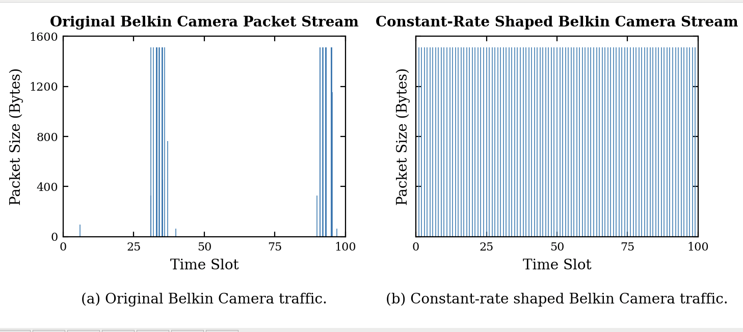
- Constant-Rate: This shaper takes an incoming packet into a memory buffer and then sends it out such that packets coming before and after it have the same constant timing. An example of this is illustrated below:
- Exponential-Rate: This shaper sources the interarrival timing from an exponential distribution instead, introducing a component of randomness.
The same traffic was shaped by the two shapers, as shown in a 30-minute unseen sample from a smart Belkin Camera. Since the model considers a sample to be every 15-minute window, the 30-minute input sample was split into two separate windows for identification.
¶ Traffic Shaping Results
-
¶ Constant-Rate shaped traffic:
-
First Window: Belkin Camera correctly predicted with ~58.05% confidence
- Top Trailing Classes and Confidence:
- Canary Camera: 16.29%
- Nest DropCam: 10.36%
- Belkin Wemo Motion Sensor: 3.33%
- Netatmo Welcome: 1.89%
- Top Trailing Classes and Confidence:
-
Second Window: Belkin Camera correctly predicted with ~47.29% confidence
- Top Trailing Classes and Confidence:
- Canary Camera: 35.61%
- Nest DropCam: 8.58%
- Belkin Wemo Motion Sensor: 1.99%
- Nest Protect Smoke Alarm: 1.85%
- Top Trailing Classes and Confidence:
-
-
¶ Exponential-Rate shaped traffic:
-
First Window: Belkin Camera correctly predicted with ~41.56% confidence
- Top Trailing Classes and Confidence:
- Canary Camera: 18.77%
- Nest DropCam: 10.38%
- Philips Hue: 4.73%
- Nest Protect Smoke Alarm: 4.67%
- Top Trailing Classes and Confidence:
-
Second Window: Belkin Camera correctly predicted with ~48.05% confidence
- Top Trailing Classes and Confidence:
- Canary Camera: 36.18%
- Nest DropCam: 8.08%
- Nest Protect Smoke Alarm: 1.85%
- Withings Sleep Sensor: 1.79%
- Top Trailing Classes and Confidence:
-
Overall, the model still predicts the correct device, albeit with a confidence level akin to a coin flip. However, the top classes consistently predicted include security cameras such as the Canary Camera and Nest DropCam, similar to the Belkin Camera. This can be attributed to the fact that packet size might be the best feature for cameras, as the device sends higher-volume traffic when it detects more objects, such as a human.
¶ Week 9: Model Refining (Presentation)
This week, the previous CNN and LSTM sequential models were retested on the new 200-day dataset; however, they remained significantly inferior to the Random Forest model.
¶ Feature Selection
Since adding statistics on Inter-arrival timing as features, the feature space has grown by 2x. This introduced a high cost in training time and may contribute to the model overfitting. To mitigate this, feature permutation and SHAP values were used to assess feature importance.
After running the feature-importance algorithms, the least important features were related to UDP-sent packets. This is most likely because devices that use UDP are less common than those that use TCP. So not all UDP features were immediately thrown out. The UDP features derived from Inter-arrival timing were removed because the distributions were highly sparse, yielding weak statistical signals. This reduced the feature space from 32 features to 24 total features.
This reduction did not significantly impact the traffic-shaping predictions or the model's overall accuracy.
¶ Traffic Shaping
A new traffic shaping experiment was tested against the fingerprinting model. The shaper randomly altered the timing and size of packets sent by an Amazon Echo over 75 minutes. After evaluating the shaper against the model, the model correctly predicted the device but with a suspiciously high confidence of ~100%. This raised suspicions, since perturbing both size and timing should have a greater impact on the model's predictions than altering timing alone.
This high performance was attributed to accidentally leaking data from using the same sample for both training the model and applying the shaper. Thus, this result was omitted from the final results.
¶ Week 10: Final Week (Final Presentation)
The final week of the project, before creating the poster and final presentation, was spent further refining the fingerprinting model and testing against traffic shapers.
¶ Model Reworks
Window sizes for the model were evaluated over the ranges 1 - 59 seconds and 1 minute - 20 minutes to choose the optimal observation time, since passive attackers wouldn't want to capture data for too long, such as 15 minutes. We measured overall accuracy against each window size plotted below:
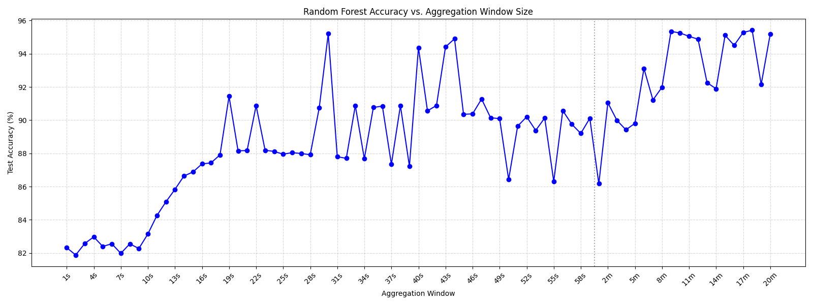
As we can see, there is still decent accuracy hovering around ~90% with a significantly shorter listening time. Thus, we decided to use 45 seconds as our window time.
Additionally, another major rework included grouping low sample devices into a class named "Unknown."
¶ Traffic Shaping
The final shaped traffic sample tested was of a 10-minute Amazon Echo sample shaped with a Constant-Rate shaper. The results are aggregated across all samples:
- Predicted Device: Amazon Echo, Confidence: 92.79%
The model is still able to correctly guess the device from the shaped traffic with good confidence.
The rest of this week and week 11 were spent preparing for the open house.
¶ Results/Conclusions
¶ Device Fingerprinting Models
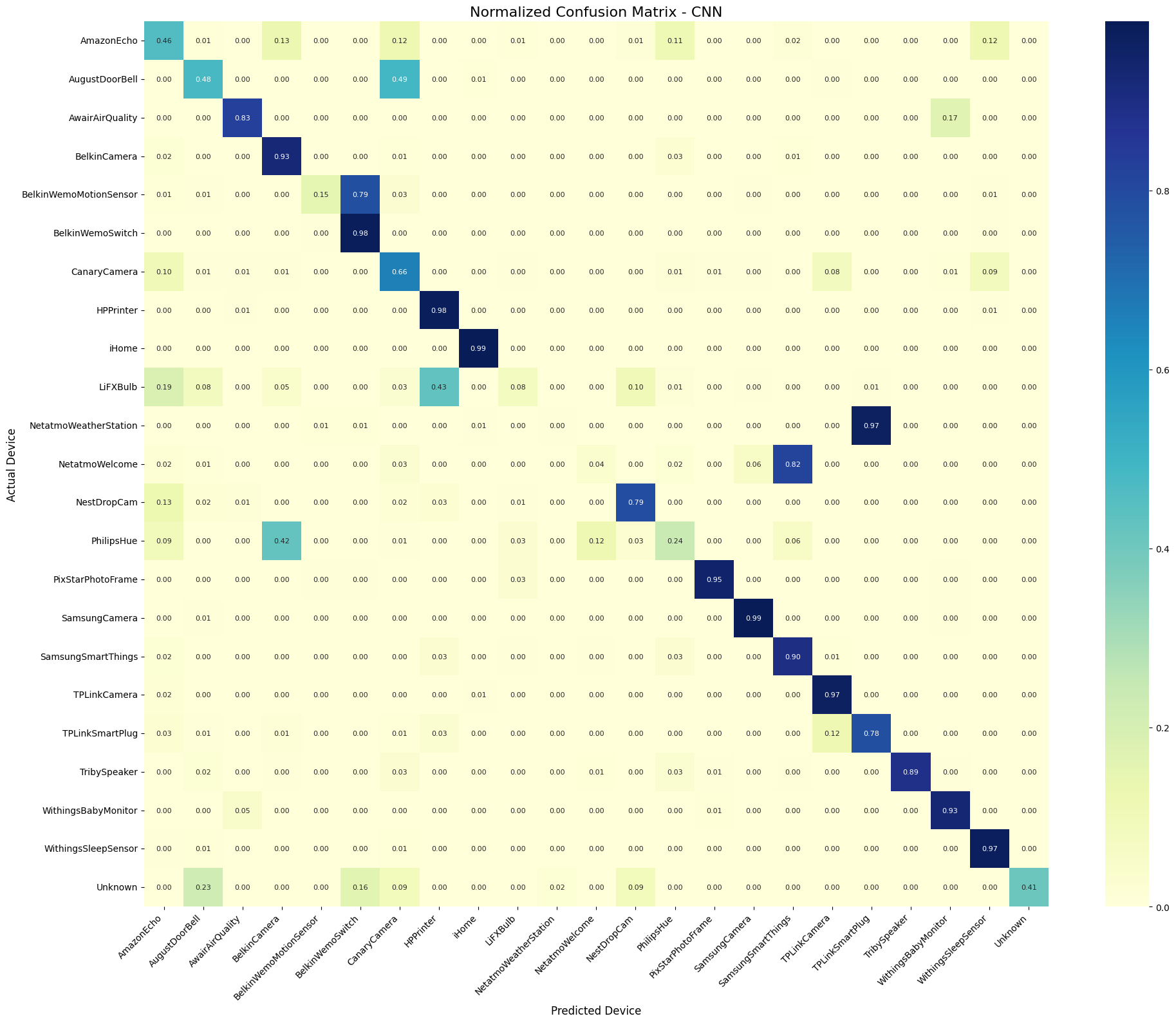
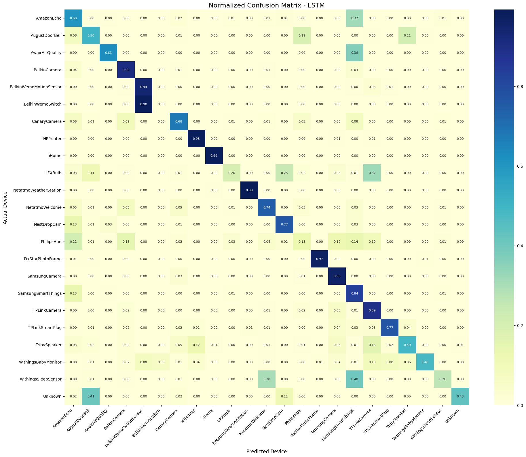
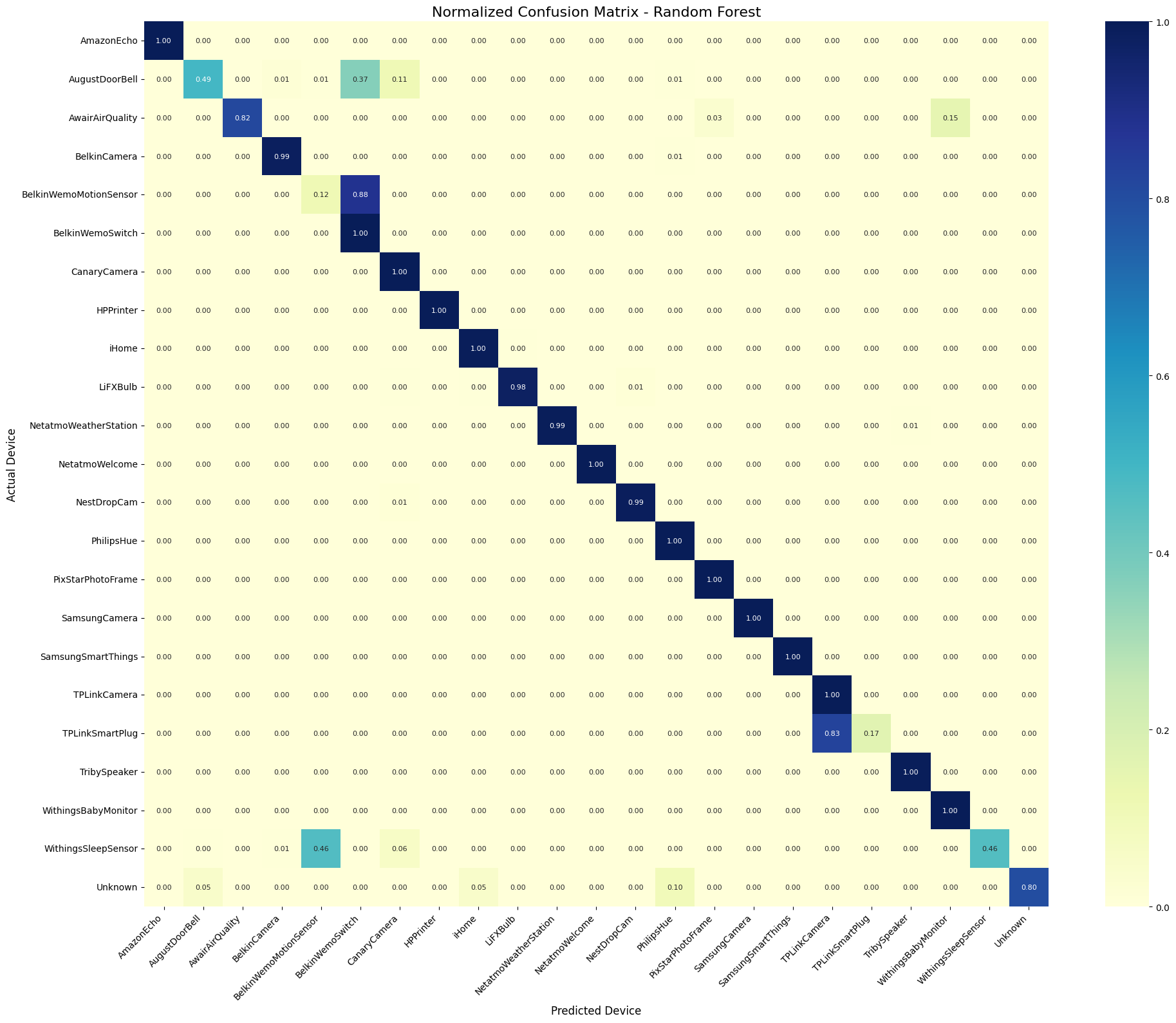
These are the final performance ratings of the device fingerprinting models. The confusion matrices show which devices are most misclassified and by how much.
¶ CNN
¶ LSTM
¶ Random Forest
¶ Model Comparison
Below are the metric comparisons of all 3 fingerprinting models:
| Model | Accuracy | Weighted F1 Score |
|---|---|---|
| CNN | 69% | 0.66 |
| LSTM | 66% | 0.64 |
| Random Forest | 88% | 0.89 |
Based on the above metrics and the confusion matrices, the Random Forest model significantly outperforms the CNN and LSTM neural network fingerprinting models, which motivated our selection of the Random Forest model as our final device fingerprinting model for testing.
¶ Traffic Shaping Results
| Device Name | Unshaped Confidence | Shaper | Confidence |
|---|---|---|---|
| Belkin Camera | 97.34% | Constant-Rate | 79.17% |
| Belkin Camera | 97.34% | Exponential-Rate | 76.71% |
| Amazon Echo | 99.82% | Constant-Rate | 92.79% |
Above is the consolidated table of all traffic-shaping experiments tested on the final device fingerprinting model. As we can see, shaping has a noticeable effect on the passive attacker, with a dip in confidence across all experiments when the model sees the same traffic unshaped.
Though this is only tested with shapers that alter inter-arrival timing, shapers that alter both would definitely create a more significant effect and a higher likelihood of misclassifications.
¶ Future Work
- Test more complex shapers that alter both packet timing AND packet size
- Test user activity inference along with device fingerprinting
- Test interleaved traffic from multiple devices as data points to simulate more realistic network traffic conditions