¶ Geo2SigMap — Getting Started with RF Signal Mapping and Sionna RT
Generate a 3D scene from geographic data for a COSMOS testbed area and compute a coverage map using the Geo2SigMap framework and the Sionna RT ray tracer.
¶ Overview
Geo2SigMap is an open-source framework for high-fidelity RF signal mapping that combines geographic databases, LiDAR terrain data, ray tracing, and a cascaded U-Net machine-learning model. It provides an automated, scalable pipeline that generates 3D building and path-gain (PG) maps from GPS-bounded areas of interest.
The repository is split into two partitions:
- Scene Generation — a pure Python pipeline that builds 3D scenes for arbitrary geographic areas, optionally enhanced with LiDAR terrain data and building-height calibration from Digital Elevation Models (DEMs).
- ML-based Propagation Model — signal-coverage prediction using a pre-trained cascaded U-Net model described in the Geo2SigMap paper.
This getting-started tutorial covers the scene-generation partition and shows how to drive Sionna RT (NVIDIA's open-source differentiable ray-tracing library) to produce a radio coverage map for a portion of the COSMOS testbed in New York City.
¶ Learning outcomes
After completing this tutorial you will be able to:
- Install Geo2SigMap and its dependencies in a Conda environment.
- Use the
scenegenCLI tool to generate a 3D scene from GPS bounding-box coordinates. - Load and preview a geo-referenced scene in Sionna RT.
- Configure a gNB transmitter and UE receiver with 3GPP TR 38.901 antenna patterns.
- Compute and visualize a radio coverage map (path gain) over a 1 km × 1 km area.
- Cite Geo2SigMap correctly in academic work.
¶ At a glance
| Difficulty | Intermediate |
| Estimated time | 60–90 min (excluding GPU setup) |
| Domain / sandbox | Any node with a GPU and internet access; example coordinates target the COSMOS testbed area in NYC |
| Topic group | Digital Twins |
| Last verified | Not re-tested (migrated 2026-06-20) |
¶ Prerequisites
Background knowledge
- Python 3.12 and Conda/Anaconda package management.
- Basic familiarity with Jupyter Notebooks (the upstream examples are notebooks).
- Basic RF / propagation concepts (carrier frequency, path gain, coverage maps).
- Familiarity with Sionna RT is helpful but not required — see the Sionna RT Technical Report and Sionna RT tutorials.
Account & access
- A COSMOS account — register here.
- An approved reservation on a domain with a GPU-equipped node — see Make a reservation.
- SSH access to the domain console — see SSH access.
¶ Resources required
Devices / nodes
| Resource | Role | Qty | Notes |
|---|---|---|---|
| GPU-equipped node | Scene generation and ray-tracing compute | 1 | RT cores recommended; CPU-only is possible but limits performance. |
Disk images
| Image | Load onto | Provides |
|---|---|---|
| TODO: verify | GPU node | Base OS with Conda/Python available; GPU drivers required for Sionna RT |
Software components
| Component | Version | Source |
|---|---|---|
| Python | 3.12 | Conda (conda-forge) |
| PDAL | latest compatible | Conda (conda-forge), installed in Conda environment |
| pyvista | 0.45.2 | pip |
| geo2sigmap | latest (v2.0.0+ as of Nov 2025) | GitHub via pip install . |
| osmnx | ≥ 2.0.0 | pip (installed as geo2sigmap dependency) |
| numpy | latest | pip (dependency) |
| pyproj | latest | pip (dependency) |
| shapely | latest | pip (dependency) |
| rasterio | latest | pip (dependency) |
| tqdm | latest | pip (dependency) |
| pillow | latest | pip (dependency) |
| open3d | latest | pip (dependency) |
| mitsuba | latest compatible | pip (dependency of Sionna RT) |
| Sionna RT | latest | pip (see Sionna docs) |
Spectrum / RF / special
Not applicable. This tutorial performs software-only ray-tracing simulation; no physical RF transmission or testbed radio hardware is used.
¶ Topology
This tutorial is software-only. All computation runs on a single GPU-equipped node. The "scene" is a geo-referenced 3D model of real-world buildings and terrain derived from public geographic databases (OpenStreetMap building footprints, LiDAR point clouds, Digital Elevation Models). Sionna RT performs ray tracing within that scene to compute path-gain values across a grid.
No SDR hardware, over-the-air transmission, or inter-node communication is involved.
¶ Setup
-
Reserve the resources (see Prerequisites) and log into the console:
ssh <username>@console.<sandbox>.cosmos-lab.org -
SSH into the GPU node:
ssh root@<gpu-node> -
Create the Conda environment with PDAL and Python 3.12:
conda create --yes --name g2sm --channel conda-forge pdal python=3.12 conda activate g2sm pip install pyvista==0.45.2 -
Clone and install the geo2sigmap package:
git clone https://github.com/functions-lab/geo2sigmap cd geo2sigmap/package pip install .The package is now installed and available via the
scenegenCLI tool or the Python function API.
The installation process should install all required packages. If you need to install them manually, the pinned pip requirements (via pipreqs, as of 1/21/2025) are:
osmnx >= 2.0.0
numpy
pyproj
shapely
rasterio
tqdm
pillow
open3d
¶ Instructions
¶ Step 1 — Find your GPS bounding box
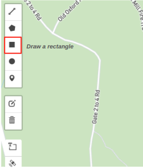
Scene boundaries are defined by parameterized GPS coordinates (min-lon, min-lat, max-lon, max-lat). Use bboxfinder.com to locate your target area: zoom to the area, click the box icon to draw a rectangle, and copy the four coordinates.
The following coordinates map a portion of the COSMOS testbed in New York City:
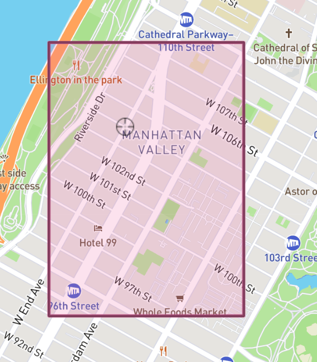
-73.973178 40.793488 -73.963824 40.803430
¶ Step 2 — Generate the 3D scene
In your working directory, run the scenegen CLI tool with the bounding-box coordinates. The --enable-lidar-terrain flag adds LiDAR terrain data for an accurate, calibrated terrain map:
scenegen bbox -73.973178 40.793488 -73.963824 40.803430 --data-dir scene/COSMOS --enable-lidar-terrain
This produces the scene files under scene/COSMOS/, including scene.xml for Sionna RT.
¶ Step 3 — Load and preview the scene
Start a Python session (or Jupyter Notebook) and run the core imports:
# Core imports
import numpy as np
import mitsuba as mi
from sionna.rt import load_scene, Transmitter, Receiver, RadioMapSolver, transform_mesh
Load and interactively preview the scene:
import os
SCENE_FOLDER = "../scene/COSMOS"
scene = load_scene(f"{SCENE_FOLDER}/scene.xml")

# Interactive 3D visualization and view of the scene
scene.preview();
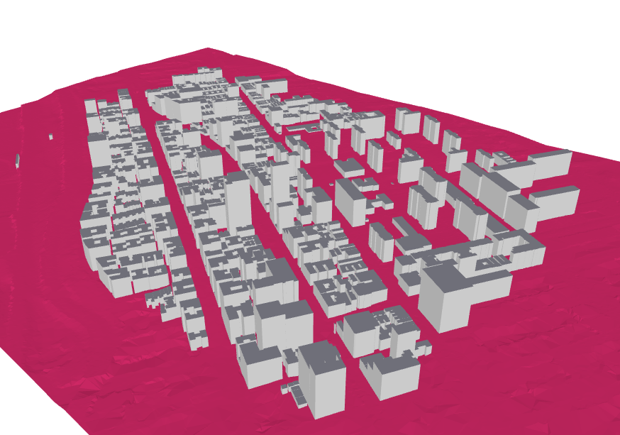
Use the left-click button and scroll wheel to explore the scene.
¶ Step 4 — Configure transmitter and receiver
This example uses the built-in 3GPP TR 38.901 antenna pattern for the gNB transmitter at 3.7 GHz (5G n48 band). The UE receiver uses an isotropic pattern:
from sionna.rt import AntennaArray
from sionna.rt.antenna_pattern import antenna_pattern_registry

# Set the operating frequency (n48 band for 5G)
scene.frequency = 3.7e9  # 3.7 GHz

# Define Rx position
ue_position = [20.0, 20.0, 0.0]   # Rx position (x, y, z in meters)

# Define Tx position
gnb_position = [0.0, 0.0, 70.0]

# gNB antenna: 3GPP TR 38.901 pattern (AIRSTRAN D 2200)
gnb_pattern_factory = antenna_pattern_registry.get("tr38901")
gnb_pattern = gnb_pattern_factory(polarization="V")

# Use isotropic antenna pattern
ue_pattern_factory = antenna_pattern_registry.get("iso")
# Polarization should match the transmitter
ue_pattern = ue_pattern_factory(polarization="V")

# SISO: Single antenna element at origin [0, 0, 0] for both TX and RX
single_element = np.array([[0.0, 0.0, 0.0]])  # Shape: (1, 3)

# Configure antenna arrays
scene.tx_array = AntennaArray(
    antenna_pattern=gnb_pattern,
    normalized_positions=single_element.T  # Shape: (3, 1)
)

scene.rx_array = AntennaArray(
    antenna_pattern=ue_pattern,
    normalized_positions=single_element.T  # Shape: (3, 1)
)

# Create Rx
rx = Receiver(name="ue", position=ue_position, display_radius=0.03)
scene.add(rx)

# Create Tx
tx = Transmitter(name="gnb", position=gnb_position, display_radius=0.03)
scene.add(tx)
¶ Step 5 — Generate and visualize the coverage map
rm_solver = RadioMapSolver()

# Create a measurement surface by cloning the terrain
# and elevating it by 1.5 meters
measurement_surface = scene.objects["ground"].clone(as_mesh=True)
transform_mesh(measurement_surface,
            translation=[0,0,1.5])

rm = rm_solver(scene,
    max_depth=5,
    los=True,
    refraction=False,
    cell_size=(1.0, 1.0),
    size=[1000, 1000],          # Size of the radio map in meters. The number of cells in the x and y directions should be [size/cell_size]
    # orientation=[0, 0, 0],    # Orientation of the radio map plane
    measurement_surface=measurement_surface, # TO BE UDPATED
    # center=[0, 0, 1.5],       # Center of the radio map measurement plane
    precoding_vec=None,
    samples_per_tx=int(1e8)
)

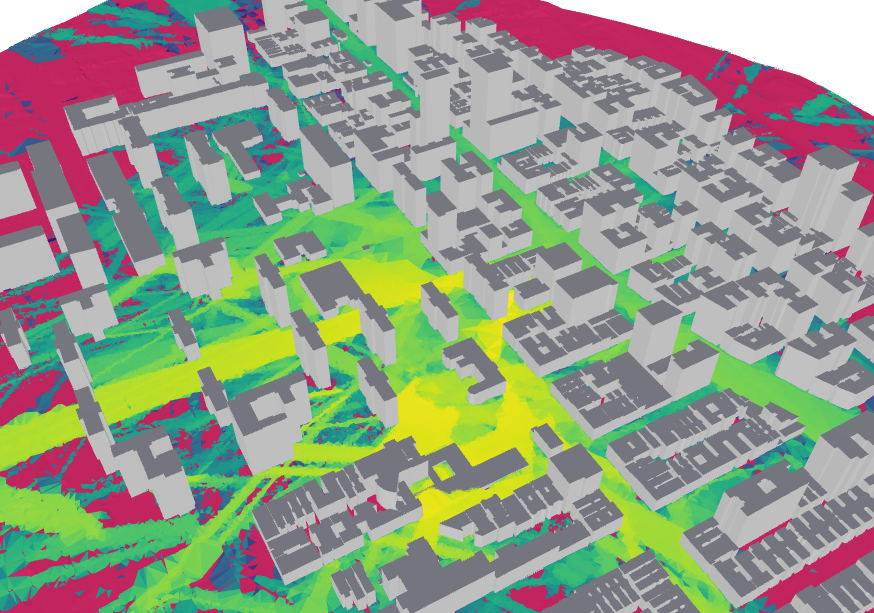
scene.preview(radio_map=rm, rm_db_scale=True, rm_metric="path_gain");
¶ Step 6 — Experiment with transmitter and receiver positions
As a simple modification, adjust the positions of the transmitter and receiver by changing these lines before re-running the entirety of the code:
# Define Rx position
ue_position = [20.0, 20.0, 0.0]   # Rx position (x, y, z in meters)

# Define Tx position
gnb_position = [0.0, 0.0, 70.0]
Note: Sionna RT does not allow re-initialization of Transmitters or Receivers if they already exist in memory. Re-run all cells from Step 4 onward to apply changes.
¶ Verification
- The
scenegencommand completes without errors and createsscene/COSMOS/scene.xmlalong with supporting mesh and material files. scene.preview()renders a recognizable 3D model of the target area (buildings visible as distinct objects, terrain surface present).- The
RadioMapSolverrun completes andscene.preview(radio_map=rm, ...)displays a color-coded path-gain map across the 1 km × 1 km area, with lower path gain (deeper shadow) behind buildings relative to the transmitter.
¶ Cleanup
This tutorial runs entirely on a single node with no persistent testbed state changes. When finished:
omf tell -a offh -t system:topo:allres
No omf save is required unless you modified the node's disk image.
The Conda environment can be removed to free disk space:
conda deactivate
conda remove --name g2sm --all
¶ Troubleshooting
| Symptom | Likely cause | Fix |
|---|---|---|
conda: command not found |
Conda not installed or not on PATH | Install Anaconda/Miniconda; source the shell init script (conda init bash) |
pip install . fails on open3d or rasterio |
Missing system libraries | Install OS-level dependencies (e.g. apt install libgdal-dev) before pip |
scenegen bbox ... fails with a network error |
Geographic data download failed | Check internet connectivity from the node; retry — OpenStreetMap/USGS servers can be intermittent |
scene.preview() produces a blank or empty window |
No display available (headless node) | Run in a Jupyter Notebook with an X11-forwarded session, or use scene.render(...) to save an image file instead |
Sionna RT RadioMapSolver runs very slowly |
CPU-only execution | Ensure a CUDA-capable GPU is available and that the correct GPU-enabled mitsuba/sionna packages are installed |
ValueError: Transmitter/Receiver already exists |
Re-running Step 4 without restarting the kernel | Restart the Python kernel and re-run all cells from Step 3 onward |
¶ References
- Geo2SigMap GitHub repository
- Geo2SigMap README / CLI documentation
- Sionna RT coverage map notebook
- Geo2SigMap paper — IEEE DySPAN 2024
If you use Geo2SigMap in your research, please cite:
@inproceedings{li2024geo2sigmap,
  title={Geo2SigMap: High-fidelity RF signal mapping using geographic databases},
  author={Li, Yiming and Li, Zeyu and Gao, Zhihui and Chen, Tingjun},
  booktitle={Proc. IEEE International Symposium on Dynamic Spectrum Access Networks (DySPAN)},
  year={2024}
}
- Sionna RT Technical Report (arXiv)
- Sionna RT tutorials
- bboxfinder.com — GPS bounding-box tool
- conda installation guide
- pipreqs
Author(s): COSMOS team · Last verified: Not re-tested (migrated 2026-06-20) · Tested image/release: TODO: verify · Tags: digital-twins, geo2sigmap, sionna, ray-tracing, coverage-map, rf-propagation, machine-learning