¶ PSK BER — BPSK / QPSK / 8PSK
Measure bit-error-rate versus Eb/N0 for phase-shift keying on two USRP B210 radios with stock GNU Radio 3.10, then overlay your measured curve on closed-form AWGN theory. This is the first modulation family of the Two-Node Digital-Modulation BER framework.
¶ Overview
Phase-shift keying encodes bits in the carrier phase: BPSK (1 bit/symbol), QPSK (2 bits/symbol), 8PSK (3 bits/symbol). Their BER-vs-Eb/N0 behavior is the textbook entry point to digital-communication measurement — BPSK and QPSK share the same theoretical curve, and 8PSK trades ~3.6 dB of power efficiency for the extra bit. This tutorial reproduces those curves on a real COSMOS link.
Two B210-equipped nodes are driven from the domain console with cosmos-ansible: the code is staged identically on both, the first node transmits an RRC-shaped PSK waveform, the second captures and recovers it (AGC → FLL → RRC matched filter → Gardner symbol sync → optional equalizer → Costas loop) and counts bit errors against a known PN sequence. Every run writes a SigMF description that a single generic plotter (sdr_plot.py) turns into a BER graph.
The shared model, the three domains (grid / sb4 / sb5), and the two SNR-sweep methods are documented once on the framework page — read Two-Node Digital-Modulation BER first. This page covers what is specific to PSK and walks one run end-to-end.
Source (clone & run): https://gitlab.orbit-lab.org/tutorials/ber
¶ Learning outcomes
After completing this tutorial you will be able to:
- Reserve two B210 nodes and run a headless two-node PSK link from a domain console.
- Sweep Eb/N0 and measure BER for BPSK, QPSK, and 8PSK.
- Explain why BPSK and QPSK share one theoretical curve and 8PSK does not.
- Produce a measured-vs-theory BER plot from the SigMF output.
- Choose between the noise-injection (ideal-AWGN) and physical-sweep (real-link) methods.
¶ At a glance
| Difficulty | Intermediate |
| Estimated time | 45 min |
| Domain / sandbox | grid, sb4, or sb5 (any two-B210 domain) |
| Topic group | SDR & GNU Radio |
| Last verified | 2026-07-20 (grid, node18-19→node18-2, 2 GHz, fresh 3-method curves) |
¶ Prerequisites
Background knowledge
- Digital modulation basics (constellations, Eb/N0, BER).
- Running a headless flowgraph — see the SDR & GNU Radio tutorials.
- The shared framework: Two-Node Digital-Modulation BER.
- COSMOS SDR hardware: SDR hardware.
Account & access
- A COSMOS account — register here.
- An approved reservation on the domain above — see Make a reservation.
- SSH access to the domain console — see SSH access.
¶ Resources required
Devices / nodes
| Resource | Role | Qty | Notes |
|---|---|---|---|
nodes[0] (e.g. node18-19 on grid) |
transmitter | 1 | USRP B210, selected first in OMF_NODES |
nodes[1] (e.g. node18-2 on grid) |
receiver | 1 | USRP B210, selected second in OMF_NODES |
The TX/RX node pair per domain (and their B210 serials) is listed on the framework page; nodes[0] is always TX, nodes[1] always RX.
Disk images
| Image | Load onto | Provides |
|---|---|---|
ubuntu2404-uhd4.9-gr3.10.ndz |
both nodes | UHD 4.9 + GNU Radio 3.10 (stock); xfce4 + Chrome Remote Desktop for the GRC GUI |
Software components
| Component | Version | Source |
|---|---|---|
| UHD | 4.x | preinstalled in image |
| GNU Radio | 3.10 | preinstalled in image (stock, no OOT blocks) |
run_ber.sh (one-file runner) |
— | download to the console; it fetches the rest |
Spectrum / RF / special
Open-air runs (grid) use a low-power B210 pair — keep the carrier inside an allowed ISM band and use a modest TX gain. On grid, use 2 GHz (much stronger node-to-node coupling than 2.4 GHz). Cabled domains (sb5) and the sb4 attenuator matrix are conducted, not radiated.
¶ Topology
Two B210 nodes in one domain, both reachable from that domain's console (console.<domain>.cosmos-lab.org) over the control plane. cosmos-ansible starts the transmitter on nodes[0] and the capture/measure pipeline on nodes[1]; the RF path between them depends on the domain:
- grid — open-air B210 → B210 (over-the-air channel).
- sb5 — cabled B210 pair through a fixed attenuator pad (clean conducted link).
- sb4 — B210 pair through the JFW attenuator matrix (SNR dialed in dB).
See the framework topology table for the exact node pairs and recommended method per domain.
¶ Setup
- Reserve the two nodes (see Prerequisites) and log into the console:
ssh <username>@console.<domain>.cosmos-lab.org - Image both nodes with the SDR image and power them on (grid example):
omf load -i ubuntu2404-uhd4.9-gr3.10.ndz -t node18-19,node18-2 omf tell -a on -t node18-19,node18-2 - Download the one-file runner onto the console:
wget https://www.cosmos-lab.org/trac/run_ber.sh
That is the only file you need — it fetches the experiment code, prepares everything, runs the measurement, and renders the BER graph. You only edit its CONFIG block.
¶ Instructions
¶ Step 1 — Edit the CONFIG block
Open run_ber.sh and set the values at the top to match your reservation. The defaults are the grid node18-19 → node18-2 BPSK+QPSK run:
NODES="node18-19,node18-2"   # your two reserved B210 nodes as  TX,RX
FREQ_HZ=2000000000           # carrier in Hz (2 GHz works on the grid)
MODS="bpsk,qpsk"             # bpsk,qpsk,8psk
RX_GAIN=60                   # receive gain (dB)
NSYMS=50000000               # bits per Eb/N0 step  (raise for a smoother low-BER tail)
EBN0="0:13:0.5"              # Eb/N0 sweep  start:stop:step  (dB)
Grid needs 2000000000 Hz (2 GHz) and adequate RX gain; a large NSYMS keeps the low-BER tail smooth (a point with zero errors cannot be plotted on a log axis — see Troubleshooting). For 8PSK, add 8psk to MODS and raise NSYMS (~3.6 dB less efficient than QPSK, so it needs more bits).
¶ Step 2 — Run it
bash run_ber.sh
That is the whole experiment. The script clones the code, transmits an RRC-shaped PSK waveform on nodes[0], captures a clean high-SNR reference on nodes[1], injects calibrated AWGN to hit each Eb/N0 target, counts bit errors against a known PN, and renders the curve. When it finishes, your BER graph, per-modulation CSVs, and SigMF metadata are in ~/tutorials-ber/results/ (ber_psk.svg is the plot). Re-running is safe — it reuses what it already fetched.
¶ Three ways to measure BER vs Eb/N0
There are three ways to put a BER-vs-Eb/N0 curve on the same axes, and comparing them is the most instructive part of this tutorial. All three below are BPSK on the grid over-the-air B210 pair (node18-19 → node18-2, 2 GHz):
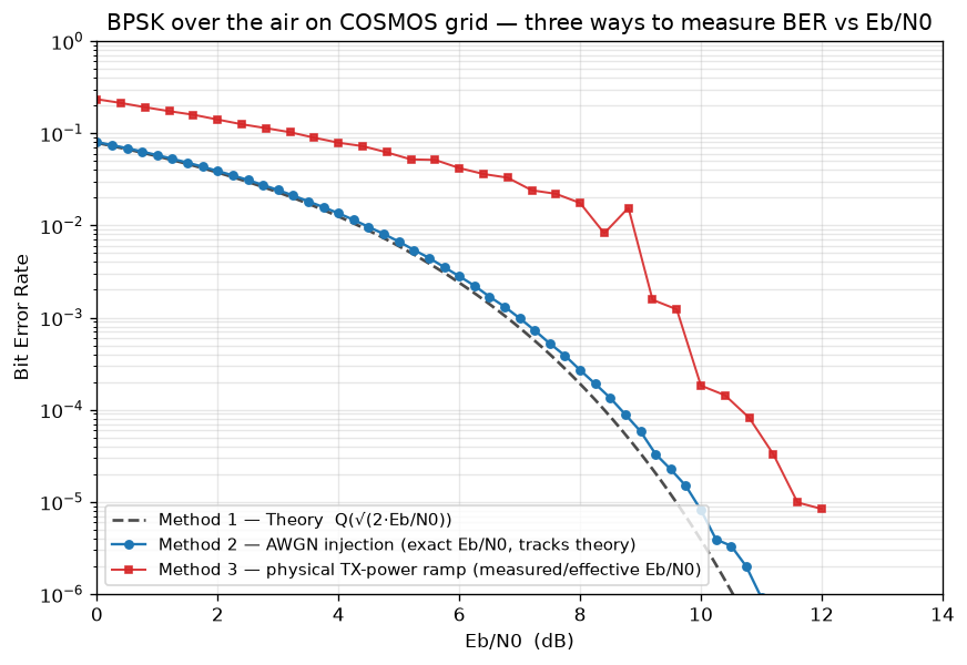
- Theory — the closed form
Q(√(2·Eb/N0)). No hardware; the reference every real curve is measured against. - AWGN injection on a real capture (the clean method) — the receiver holds one solid high-SNR lock over the real radios, then calibrated noise is added in software to hit each Eb/N0 target exactly and count errors against the known PN. Because Eb/N0 is set, not estimated, the curve is smooth all the way down to ~1e-6 and sits ~1–2 dB right of theory — the honest implementation loss of real B210s (LO phase noise, EVM, timing/carrier recovery). This is what
run_ber.shruns by default, and the curve you should reproduce. - Physical TX-power ramp (the real link) — actually walk the transmit power down while the receiver holds lock and tracks (it never re-acquires), reading BER per short window. With a large bit count the ramp is smooth all the way into the low-BER tail; the curve above is ~110 M symbols per run, weighted so the low-BER end gets the most bits. It sits several dB right of the injection curve — see below.
¶ Why the ramp sits right of theory — the Eb/N0-calibration problem
The ramp is smooth, but its x-axis is not the same quantity as method 2's. Over the air you cannot set Eb/N0 — you have to estimate it from the received symbols, and that estimate is the effective Eb/N0: AWGN plus the hardware EVM (LO phase noise, timing jitter). Because EVM adds to the error, the estimated Eb/N0 reads a few dB optimistic and the whole ramp shifts right of theory. Method 2 sidesteps this entirely: it injects a known amount of AWGN, so its x-axis is exact and the curve rides theory to ~1 dB. So the smoothness knob is bit count (the user's rule: many bits per step at high SNR), but the honest absolute Eb/N0 comes from injection — the ramp shows the real link's shape, injection places it precisely on the axis. (Both are correct; they measure different x-axes.)
QPSK behaves like BPSK here: equal per-bit BER, a hair more sensitive to residual phase error. This small, roughly constant PSK gap contrasts with the QAM page, where the gap is much larger and grows with SNR because the dense QAM constellation is far more EVM-sensitive.
¶ Open the flowgraphs in GNU Radio Companion (GUI)
The transmit and receive chains are also provided as GNU Radio Companion flowgraphs — grc/ber_tx.grc and grc/ber_rx.grc in the repo — for interactively watching the receiver lock: the RX flowgraph shows the recovered constellation snapping to the BPSK/QPSK points and the live spectrum. They are the GUI counterpart of the headless tx.py/rx.py; switch BPSK↔QPSK by editing the single const variable block (default BPSK).
GRC is a graphical application, so you need a remote desktop to the node — a plain SSH session cannot display it. The ubuntu2404-uhd4.9-gr3.10.ndz image ships xfce4 + Chrome Remote Desktop preinstalled for exactly this. Two ways to get a desktop on the node:
- Chrome Remote Desktop (recommended) — enroll the node once with your Google account, then open its xfce desktop in a browser. Setup: Chrome Remote Desktop.
- Remote X / X11 forwarding — forward the display over SSH. Setup: Remote Graphics.
Then, from a terminal in the node's desktop:
gnuradio-companion ~/ber/grc/ber_rx.grc # opens the RX flowgraph; press ▶ Run
Start ber_tx.grc on the TX node and ber_rx.grc on the RX node. The GRC flowgraphs are for interactive exploration; for the swept BER measurement use the headless tx.py/rx.py via the playbooks above.
¶ Verification
A successful run produces a measured BER curve (Method 2 above) that rides theory within ~1–1.5 dB. These are the actual BPSK injection points from the grid node18-19 → node18-2 link (2 GHz, capture at ~21 dB real Eb/N0, then calibrated AWGN, 12 M bits/point):
| Eb/N0 (dB) | measured BER | theory Q(√(2·Eb/N0)) |
|---|---|---|
| 0.0 | 8.03e-2 | 7.86e-2 |
| 3.0 | 2.42e-2 | 2.29e-2 |
| 6.0 | 2.81e-3 | 2.39e-3 |
| 8.0 | 2.69e-4 | 1.91e-4 |
| 9.0 | 5.83e-5 | 3.36e-5 |
| 10.0 | 8.17e-6 | 3.87e-6 |
| 11.0 | 9.17e-7 | 2.61e-7 |
What to look for:
- Markers track the dashed theory line with ~1–1.5 dB of implementation loss — exactly what ideal-AWGN injection on real B210s should show. QPSK lands on the same curve (two orthogonal BPSK streams — same per-bit BER, twice the data rate).
- The tail stays smooth down to ~10⁻⁶ because of the large bit count. This is the key knob: at high Eb/N0 the BER is tiny, so you need many bits per point or the curve turns jagged / floors — a point with zero errors cannot be plotted on a log axis. Raise
NSYMSto push the smooth tail deeper.
¶ Cleanup
# Nothing to save — the image is unmodified. Just free the nodes:
omf tell -a offh -t node18-19,node18-2
Release the reservation from the portal when finished.
¶ Troubleshooting
| Symptom | Likely cause | Fix |
|---|---|---|
No UHD Devices Found |
node ↔ B210 USB not enumerated | power-cycle the node (omf tell -a offh then on); confirm uhd_find_devices on the node |
| BER floors flat at a nonzero value | link too weak to reach the low-BER tail | raise ber_rx_gain; on grid use ber_freq_hz=2000000000 (2 GHz), not 2.4 GHz |
| Curve stops early / missing low-BER points | too few bits (zero-error points can't be plotted on log axis) | raise ber_nsyms (e.g. 50 M+ for BPSK/QPSK) |
ber_psk.svg empty or missing a series |
no .sigmf-meta for that modulation in results/ |
re-run the family; confirm PLAY RECAP had failed=0 and the fetch step ran |
| Injection curve beats theory | impossible — capture was not clean AWGN | injection needs a high real-link Eb/N0; use a stronger link before injecting |
¶ References
- Framework overview & settings: Two-Node Digital-Modulation BER
- Repo (clone & run): https://gitlab.orbit-lab.org/tutorials/ber
- Shared setup: Make a reservation · SSH / console · SDR hardware
- Interactive IQ viewer (for
.sigmf-datacaptures): IQEngine - SigMF specification: https://github.com/sigmf/SigMF
Author(s): COSMOS team · Last verified: 2026-07-18 (grid, node18-19/node18-2, 2 GHz, noise-injection; real-link sweep path re-verified 2026-07-19) · Tested image/release: ubuntu2404-uhd4.9-gr3.10.ndz / GNU Radio 3.10.12 · Tags: sdr, gnuradio, ber, psk, bpsk, qpsk, sigmf