¶ OFDM Bit Error Rate at FR1 (sub-6 GHz) — a three-mechanism laboratory
Measure the bit error rate of a real OFDM link on COSMOS at 2.4 GHz — sub-6 GHz, or FR1 in 3GPP's naming — three different ways, and learn why the three do not agree about what is easy to measure. You will add calibrated noise to a cabled link, attenuate a real signal path with a programmable matrix, and walk the transmit power of an over-the-air link — then compare BPSK, QPSK and 8-PSK on each.
¶ Overview
Looking for FR3, or for 16-QAM and 64-QAM? They are on the companion page, OFDM BER across five subcarrier modulations. The two pages divide the material by method, not only by band: this one gives you an interactive flowgraph and compares three ways of moving the operating point, all at FR1. That one is an automated sweep across all five subcarrier modulations, and runs on the sb1 FR3 chain or on the same FR1 hardware used here.
A bit error rate (BER) is the simplest possible statement about a digital radio link: of every million bits sent, how many arrived wrong? A waterfall curve plots that against signal-to-noise ratio, and it is the single most common figure in a digital communications course, because its shape encodes almost everything about a modulation scheme.
Textbook waterfalls are computed. This laboratory measures one, on hardware, and the difference is the point of the exercise. Three things will happen that no simulation shows you:
-
The transmitter can be driven too hard. OFDM sums many subcarriers, so its peak-to-average power ratio is high and the transmit chain clips on peaks long before its average power looks excessive. A clipped OFDM transmitter produces a few percent BER and — the diagnostic detail — not one perfect packet. You will measure the drive window before measuring anything else, because every later number depends on being inside it.
-
The measurement has its own floor. Adding noise to a link can only make it worse down to the noise the receiver already has. Ask for a signal-to-noise ratio higher than the link's own margin over thermal noise and the sweep quietly measures the link instead of your injected noise, returning a plausible number the whole way. The curve flattens, and the flat part looks exactly like a property of the modulation. It is not.
-
Frame synchronisation gives out before bit decisions do. Below roughly 9 dB of SNR this receiver stops finding packet headers at all. No payload is emitted, so there is no BER to compute — not a high BER, an absent one. The usable floor of the whole system is set by the frame detector, not by the bit detector.
Each of the three mechanisms moves the operating point differently, and each has a different weakness. Running all three and comparing is what turns "I plotted a curve" into "I know what my measurement can and cannot tell me".
| Mechanism | What changes | Strength | Weakness |
|---|---|---|---|
| A — injected noise | Noise added at the receiver | Exact, repeatable, reproducible from a seed | Ceilinged by the link's own margin over thermal |
| B — path attenuation | The signal genuinely arrives weaker | No SNR ceiling; thermal noise is the noise | Needs a programmable attenuator (sb4 only) |
| C — transmit power | The transmitter drives harder | Needs no extra hardware at all | Coarse, quantised, non-linear near compression, and the low-BER end is unaffordable |
¶ Learning outcomes
After completing this tutorial you will be able to:
- Explain what a BER waterfall curve shows, and read one critically.
- Measure the transmit drive window of an OFDM link, and recognise the signature of an overdriven transmitter.
- Compute the SNR a receiver actually experiences, as distinct from the SNR a sweep was asked to produce.
- Choose between noise injection, path attenuation and transmit power for a given measurement, and justify the choice.
- Compare BPSK, QPSK and 8-PSK on identical hardware and account for the differences.
- Explain why error-free points are an upper bound rather than a measurement, and why the number of errors — not the number of bits — sets a BER estimate's precision.
¶ At a glance
| Difficulty | Intermediate |
| Band | FR1 / sub-6 GHz — 2.4 GHz ISM throughout |
| How you run it | Interactive and automated. Parts 1–2 are done by hand in GNU Radio Companion; Parts 3–5 are sweeps and run under Ansible |
| Estimated time | 60 min for one mechanism interactively; 3–4 h for the full nine-curve set with Ansible |
| Domain / sandbox | sb5 (mechanism A), sb4 (mechanism B), grid (mechanisms A and C — B210 pair for the figures here, X310 pair at 2 GHz for the better link) |
| Topic group | SDR & GNU Radio |
| Last verified | 2026-08-01 |
¶ Prerequisites
Background knowledge
- Basic digital modulation: what a constellation is, what BPSK/QPSK/8-PSK mean.
- Decibels, and the difference between a power ratio and an amplitude ratio.
- Enough GNU Radio to open a flowgraph and press play — see Getting started with GNU Radio.
- Comfort with
sshand the Linux command line.
Account & access
- A COSMOS account — register here.
- An approved reservation on whichever sandbox you use — see Make a reservation.
- SSH access to the domain console — see SSH access.
This experiment transmits. Stay inside your reservation window. On
sb4the RF matrix service accepts requests from your own account only — run the experiment as your COSMOS username, not asroot.
¶ Resources required
Devices / nodes
You need one pair, not all six. Each mechanism runs on its own sandbox, and each needs exactly two nodes. Pick the sandbox you have a reservation on; the whole laboratory can be done on any one of them, and doing all three is what lets you compare the mechanisms.
Sandbox sb5 — Mechanism A, injected noise over a cable
| Resource | Role | Notes |
|---|---|---|
node1-1.sb5 |
transmitter | USRP B210, cabled to node1-2 through a fixed 60 dB attenuator |
node1-2.sb5 |
receiver | USRP B210 |
Sandbox sb4 — Mechanism B, programmable attenuator
| Resource | Role | Notes |
|---|---|---|
node1-4.sb4 |
transmitter | USRP B205mini, RF matrix port 3 |
node1-5.sb4 |
receiver | USRP B205mini, RF matrix port 6 |
The SDR on
node1-Nis not on matrix portN. The feeds are node1-3 → ports 1/2, node1-4 → 3/4, node1-5 → 5/6, node1-6 → 7/8. For the pair above that means TX/RX on port 3 and RX2 on port 6. Only node1-3 to node1-6 carry USRPs at all.
Sandbox grid — Mechanisms A and C, over the air
| Resource | Role | Notes |
|---|---|---|
node18-2.grid |
transmitter | USRP B210, over the air |
node18-19.grid |
receiver | USRP B210, ~17 antenna positions away |
node3-1.grid |
transmitter | USRP X310, over the air — the 2 GHz option below |
node3-20.grid |
receiver | USRP X310, ~19 antenna positions away |
Disk images
| Image | Load onto | Provides |
|---|---|---|
baseline-sdr.ndz |
every node used | UHD 4.9 and GNU Radio 3.10, preinstalled |
Always use the
baseline-sdr.ndzsymlink, never its versioned target. The symlink is repointed when the reference image is rebuilt, so a tutorial written against it keeps working. Use the same image on both nodes of a pair: a mixed pair once cost a full day of debugging on sb4, with the same GNU Radio version but a different distro build at each end and a link that would not decode despite a perfect RF path.
Software components
| Component | Version | Source |
|---|---|---|
| UHD | 4.9 | preinstalled in the image |
| GNU Radio | 3.10.12 | preinstalled in the image |
cosmos_lab.orchestration |
0.1.0 | preinstalled on every console |
Spectrum / RF / special
2.4 GHz ISM, 1 MSps, roughly 840 kHz of occupied bandwidth. sb5 and sb4 are cabled and radiate nothing. The grid pair radiates over the air inside the shielded grid enclosure.
¶ ⚠️ 2.4 GHz is shared with Wi-Fi, and the grid room is full of it
Everything on this page runs in the 2.4 GHz ISM band, which is the same band as 802.11b/g/n — and the ORBIT grid room has a great deal of Wi-Fi in it. That matters differently depending on which sandbox you use:
sb5andsb4are cabled, as aresb6andsb7. The signal runs through coax and an attenuator — a fixed 60 dB pad onsb5andsb6, only 20 dB onsb7, and a programmable matrix onsb4— so Wi-Fi cannot get into the measurement in any meaningful way. This is why the cleanest waterfalls in this laboratory come from there, and why you should prefer them whenever you want a repeatable number.gridradiates over the air. A busy Wi-Fi channel raises the noise floor, and worse, raises it intermittently — which does not average out and does not look like thermal noise. It looks like an unstable link, or a BER floor that moves between runs for no reason.Every sweep measures the noise floor before it starts, with the transmitter off, and prints it. Use that:
text received RMS 0.020742, floor 0.00027738 -> signal RMS 0.020741 (37.5 dB above floor)Run the same experiment twice on
grid. If the floor moves by more than a decibel or two between runs, something else is transmitting and your curve is measuring it. Move to a cabled sandbox, or changefreq_hz— a B210 covers 70 MHz to 6 GHz and nothing in these experiments depends on being at 2.4 GHz.The band is used here because every radio on the testbed supports it, which makes the three sandboxes directly comparable. That is a teaching convenience, not a requirement.
¶ Moving off 2.4 GHz is not free — change the radio too
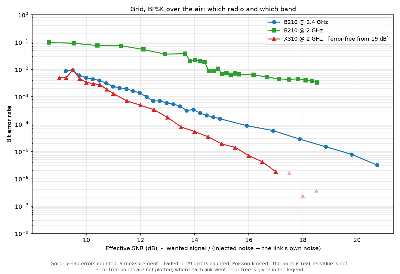
The obvious response to the warning above is to retune the grid pair away from Wi-Fi. Tried on 2026-08-03, that made the link worse:
Grid BPSK, same 7 m path, same description Signal above the receiver's own floor Best BER reached B210 @ 2.4 GHz 27.7 dB 3.2 × 10⁻⁶ B210 @ 2 GHz 19.4 dB 3.3 × 10⁻³, flat, never descends X310 @ 2 GHz 61.6 dB 0 — error-free from 19 dB
The grid antennas are 2.4 GHz types. Retuning the radio does not retune them, so 2 GHz costs more in antenna mismatch than it gains in avoided interference. The green curve is the signature: a flat plateau, not a waterfall. The link never gets far enough above its own noise for the noise you inject to be what limits it, so adding less of it changes nothing. That is a margin ceiling, and it is the single most common way a BER measurement lies to you: the curve looks like the modulation has hit its limit when what it has actually hit is the link's. Part 3 shows how to tell the two apart — the floor the sweep prints, with the transmitter off, is the number that decides it.
The X310 pair at 2 GHz is the configuration that actually works: 42 dB more margin than the B210s at the same carrier, a curve that is steeper as well as lower, and zero errors from 19 dB — which neither B210 configuration reaches anywhere. If you want the grid, off the Wi-Fi band, and clean, use
sdr/ofdm-ber-grid-x310.description.yml.The lesson generalises past this page: a link budget is a property of the whole chain, and the antenna is part of it. Changing one element to fix one problem routinely uncovers a different limit that was hiding underneath.
¶ With that margin, 64-QAM works at 2 GHz too
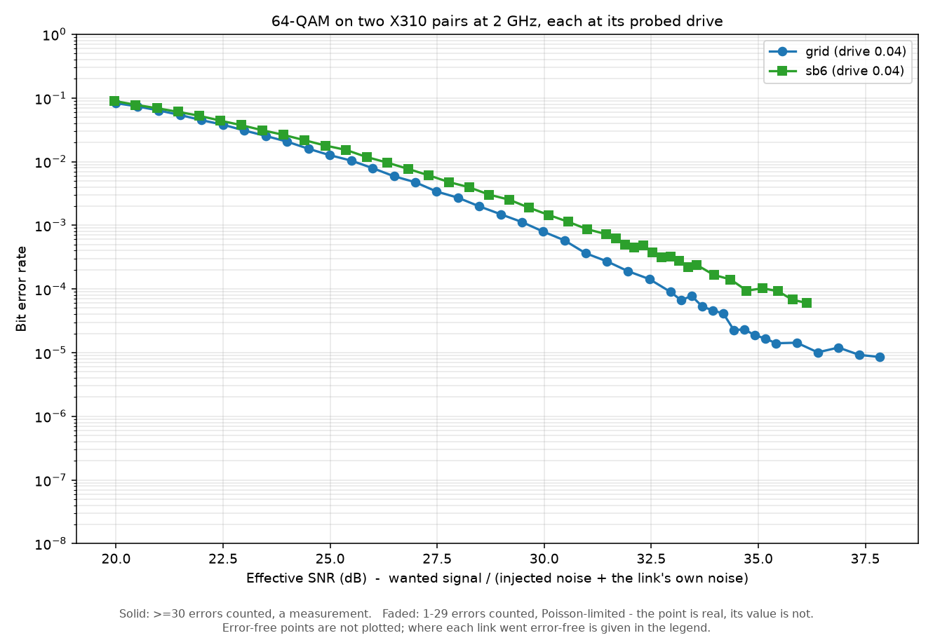
The X310 pair's headroom is not just a better BPSK number — it is enough to carry the densest constellation this laboratory offers:
64-QAM at 2 GHz, drive 0.04 Signal above own noise floor Best BER Perfect packets grid node3-1/node3-2052.3 dB 8.5 × 10⁻⁶ at 37.8 dB 23 484 / 23 511 sb6 node1-1/node1-240.7 dB 6.0 × 10⁻⁵ at 36.1 dB 4 421 / 4 476
The two curves lie on top of each other down to about 10⁻⁴ and then separate. That is not a difference between the radios. sb6 sits 40.7 dB above its own noise floor at this drive, so asking for 38 dB of effective SNR leaves it almost no headroom and the link's own noise takes over; grid has 52.3 dB. The flat tail is a margin ceiling — the same shape, and the same cause, as the green plateau above.
Two things this measurement needs, and neither is optional. 64-QAM wants its own drive — 0.04 here, against 0.15 for BPSK; at 0.15 the constellation is destroyed by transmit overdrive and the BER pins flat near 0.24 no matter what noise you add. And it wants its own SNR range: below about 27 dB it does nothing interesting, so a sweep that stops at 20 dB shows a "floor" that is only the end of the axis. Run Part 2 first, and set
snr_dbto reach at least 36 dB.-e '{"cosmos_parameters": {"sub": "64qam", "amplitude": 0.04, "snr_db": "20:38:0.5"}}' ```
¶ Topology
All three configurations are the same experiment — one node transmits a known repeating payload, the other receives it and counts bit errors — differing only in what sits between the two radios and what is varied.
  MECHANISM A - injected noise (sb5)
      node1-1 ──[ fixed 60 dB attenuator, coax ]── node1-2
                                               │
                                     AWGN added in software
                                     at the receiver, scaled
                                     to a requested SNR

  MECHANISM B - path attenuation (sb4)
      node1-4 ──[ JFW matrix, 0-95 dB in 1 dB steps ]── node1-5
                  plus ~20 dB fixed insertion loss
              port 3                                    port 6
                        the SIGNAL is attenuated;
                        thermal noise is the only noise

  MECHANISM C - transmit power (grid)
      node18-2  )))            over the air, ~17 positions            (((  node18-19
                        the TRANSMIT GAIN is stepped;
                        nothing is added to the link
¶ Setup
-
Reserve the resources and log into the console for your sandbox:
ssh <username>@console.sb5.cosmos-lab.org -
Make sure the nodes are off before imaging:
omf tell -a offh -t node1-1,node1-2 -
Load the SDR image onto both nodes:
omf load -i baseline-sdr.ndz -t node1-1,node1-2 -
Turn them on and confirm they are up:
omf tell -a on -t node1-1,node1-2 omf stat -t node1-1,node1-2 -
Check that each node came up on the image you asked for. Do this every time, on each node separately — it takes seconds and it is the difference between measuring your link and measuring someone else's leftover setup:
for n in node1-1 node1-2; do echo -n "$n: " ssh root@$n 'cat /.omf-image-name; which uhd_find_devices >/dev/null && echo " UHD present"' doneExpected:
node1-1: baseline-sdr.ndz UHD present node1-2: baseline-sdr.ndz UHD presentTwo failure modes look different and are worth telling apart:
- SSH refuses your key, but password
rootworks. The node never left
the PXE stage image. Power-cycle it:omf tell offh -t <node>, wait about
twenty seconds, thenomf tell on -t <node>. - A different image name, or no
/.omf-image-nameat all. The node is
running something else. Load it again.
- SSH refuses your key, but password
-
Confirm each node sees its own USRP:
ssh root@node1-1 'uhd_find_devices --args="type=b200" 2>&1 | egrep "type|serial|product"'On
grid, every node can also reach around twenty networked X310s. Withouttype=b200pinning the locally-attached B210, UHD is free to pick one of those — the most common wrong-SDR failure on that sandbox.
¶ Instructions
The laboratory has five parts.
Part 1 is interactive — you drive the link yourself in GNU Radio Companion, with live controls, and see every effect the rest of the laboratory measures. Do it first; nothing later means much without it.
Parts 2–5 are automated, because each is a sweep of thirty-odd operating points and a sweep is a loop, not something to type. The automated path runs the same DSP: the graphical flowgraphs are derived from the headless ones by script so the two cannot teach different things.
¶ Part 1 — Interactive: drive the link yourself in GNU Radio Companion
Open the flowgraphs and drive the link by hand — remote graphics setup, what the displays mean, and three things to try. Click to collapse.
Do this part first, and do it by hand. Everything the rest of the laboratory measures numerically, you can see here by dragging a slider — and seeing it once is worth more than the whole table of numbers that follows.
The graphical flowgraphs are the same DSP as the automated ones. They are derived from the headless pair by a script rather than maintained separately, precisely so the thing you watch and the thing that produces the curves cannot drift apart. The only additions are displays and live controls.
Interactive mode covers BPSK, QPSK and 8-PSK only. There is no graphical path for 16-QAM or 64-QAM, and that is a limitation of GNU Radio rather than of this tutorial:
digital.ofdm_txmaps 1, 2 and 3 bits per symbol and callsexit(1)on anything denser. The two QAM constellations are transmitted by a ported version of that block, which the automated parts use and which has no GRC equivalent.So do Part 1 with a PSK, and use the automated parts — 3 to 5 — for anything denser. The FR3 OFDM tutorial runs all five subcarrier modulations under Ansible, including both QAMs.
¶ Stage and open them
From the console, put the flowgraphs on both nodes:
FG=~/.ansible/collections/ansible_collections/cosmos_lab/orchestration/roles/fr3_ofdm_ber/files
for n in node1-1 node1-2; do
  ssh root@$n 'mkdir -p /run/cosmos/fr3-ofdm'
  scp $FG/grc/fr3_ofdm_tx_bpsk_gui.grc $FG/grc/fr3_ofdm_rx_bpsk_gui.grc \
      $FG/make_noise.py root@$n:/run/cosmos/fr3-ofdm/
done
The receiver's flowgraph opens its noise recording when it is constructed, whether or not any noise is being injected, so a file has to be there before you press play — a missing one kills the receiver at start-up with RuntimeError: can't open file. There are two ways to put one there.
Generate one on the node. The three stock recordings are made from a seed, so they reproduce byte-identically:
ssh root@node1-2 'cd /run/cosmos/fr3-ofdm && python3 make_noise.py noise_awgn \
  --kind=awgn --count=1048576 --seed=1 --samp-rate=1000000'
Swap --kind=awgn for coloured or impulsive to change what the noise is (see Part 3).
Or copy one you already have. Anything in raw interleaved complex64 works — a capture of a real interferer, a recording from another experiment, something a colleague sent you. Copy it from the console to the receiver:
# on the console, with the recording in your home directory
scp ~/wifi-burst.sigmf-data root@node1-2:/run/cosmos/fr3-ofdm/
and point the receiver's noise_file parameter at /run/cosmos/fr3-ofdm/wifi-burst.sigmf-data.
Two things to check on a file you did not generate:
- it must be the
.sigmf-datahalf of a SigMF pair — the.sigmf-metahalf is JSON and will not load; - its length in bytes must be a multiple of 8, or it is not interleaved complex64 and is either a different sample format or truncated.
Its absolute level does not matter. The receiver scales it by noise_scale, and the automated sweeps in Part 3 measure the recording's own RMS and scale it to hit each requested SNR — so a capture taken at any gain gives the same curve.
Under Ansible you do not copy anything by hand:
noise_filetakes a path on the console and the role validates it and ships it to the receiver for you. That is the form used in Part 3.
¶ Getting a graphical window onto your screen
GNU Radio Companion is a GUI application running on a node several hops away, so you need one of the two supported ways to see it. They are documented in full on Remote Graphics — read that page once and the rest of this section is a two-line reminder.
| Method | Best for | Setup |
|---|---|---|
| X11 forwarding | one or two windows over an SSH session you already have | Remote Graphics |
| Chrome Remote Desktop | a full persistent desktop — several windows at once, and it survives a dropped connection | Chrome Remote Desktop |
For this laboratory you open two flowgraphs at once and keep them open while you drag sliders, so a desktop is the more comfortable of the two. X11 forwarding is quicker to start if you only want a look.
With X11 forwarding — the -X flag on every hop
The flag is needed on each ssh in the chain: laptop → console → node. Miss it on either and the window has nowhere to draw.
# terminal 1 — the transmitter
ssh -X <username>@console.sb5.cosmos-lab.org
ssh -X root@node1-1 'cd /run/cosmos/fr3-ofdm && gnuradio-companion fr3_ofdm_tx_bpsk_gui.grc'

# terminal 2 — the receiver
ssh -X <username>@console.sb5.cosmos-lab.org
ssh -X root@node1-2 'cd /run/cosmos/fr3-ofdm && gnuradio-companion fr3_ofdm_rx_bpsk_gui.grc'
You also need an X server on your own machine — already present on Linux, XQuartz on macOS, VcXsrv or the WSL X server on Windows. macOS generally needs -Y rather than -X. The per-OS setup is on the Remote Graphics page.
Two windows over two SSH chains is about the limit of what this is pleasant for, and everything dies with the connection.
With Chrome Remote Desktop — a real desktop on the node
Set up per
Chrome Remote Desktop, then connect to the node's desktop from your browser. From there this is ordinary desktop work rather than SSH work — there is no -X, and no second terminal:
# in a terminal on the node's desktop
cd /run/cosmos/fr3-ofdm
gnuradio-companion fr3_ofdm_tx_bpsk_gui.grc &
gnuradio-companion fr3_ofdm_rx_bpsk_gui.grc &
Both windows sit side by side on one desktop, which is what you want when the whole point is to drag a slider in one and watch the other. The session also survives a dropped connection — reconnect and the flowgraphs are still running, which X11 forwarding will not do.
Note that CRD gives you a desktop on one machine. Running the transmitter and the receiver on their own nodes means a desktop on each, or a desktop on one and SSH to the other.
¶ What the flowgraphs look like
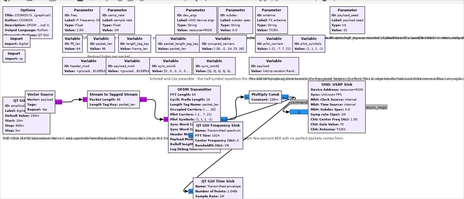
The transmitter — a Random Source feeding the stock OFDM Transmitter block, then the drive control and the USRP:
The receiver — note the File Source and Add on the left, which is where the noise recording is summed onto the received samples, ahead of frame sync:
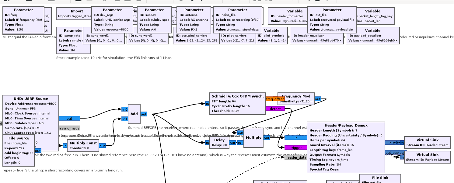
The parameter blocks along the top are what you fill in below. The block comments overlap each other on the canvas — that is cosmetic, and they are readable when you click a block.
In each window set the launch-time arguments that are not sliders — they select the radio and cannot be changed while running — then press ▶.
| Set on | Argument | Value |
|---|---|---|
| both | freq |
2.4e9 |
| both | samp_rate |
1000000 |
| both | dev_args |
type=b200 |
| both | subdev |
A:A |
| transmitter | antenna |
TX/RX |
| receiver | antenna |
RX2 |
Start the transmitter first, and give a B210 about twelve seconds before you judge anything at the receiver. It does not stream immediately, and a link looked at too early reads tens of decibels weaker than it is — which cost this project an afternoon before it was understood.
¶ What you are looking at
Transmitter window
- Transmitted spectrum — the OFDM block, about 840 kHz wide at 1 MSps.
- Transmitted envelope — the most useful display in the laboratory. OFDM sums many subcarriers, so the peaks reach far above the average level you set.
Receiver window
- Received spectrum — confirms the signal is where you think it is.
- Equalized payload symbols — the constellation the bit decision is actually made on. Two tight dots is a healthy BPSK link; a smeared cloud is noise.
Why this constellation is trustworthy. The stock decision-feedback equaliser snaps its output onto the constellation unless soft output is enabled, so a display fed from the default shows two immaculate dots on a link with 2.4e-2 BER — it looks perfect no matter how bad things are. The graphical variants turn soft output on for exactly this reason. It changes no decision and no BER; it only stops the display from lying to you.
¶ Experiment 1 — find the wall by ear, so to speak
On the receiver, drag injected noise scale up from 0.
Watch the two constellation dots grow into clouds, and the clouds move towards each other. Keep going. At some point they overlap enough that the decision boundary starts cutting through real symbols — that is the crossover region of the waterfall curve, and you are watching it happen in real time.
Push a little further and something more abrupt happens: the constellation stops updating altogether. That is not "very high BER". The receiver has stopped finding packet headers, so no payload is being emitted at all and there is nothing left to display. Everything below that point is invisible to a BER measurement — measured later in this laboratory at 8.74 dB SNR on this link and 9.23 dB on the over-the-air pair.
Back the noise off until the constellation returns.
¶ Experiment 2 — overdrive the transmitter, and watch it break
Set the receiver's noise slider back to 0. The constellation should be tight.
Now on the transmitter, raise digital drive (amplitude) from 0.15 towards 0.40, watching both windows:
- On the transmitter's envelope display, the peaks climb towards ±1 and flatten against it. That is clipping.
- On the receiver's constellation, the dots smear — even though you just made the signal stronger.
This is the single most counter-intuitive result in the laboratory: more transmit power made the link worse. Nothing at the receiver can undo it, because the damage happened in the transmitter before the signal left the node.
Then go the other way — bring the drive down to 0.03 and below. The constellation smears again, this time because there is not enough signal. The useful window is between the two, and Part 2 measures where.
Both failures produce the same headline symptom: a few percent BER with no perfect packets. That symptom alone does not tell you which one you have — only the direction of the trend does. Raise the drive: if it gets worse you were overdriven, if it gets better you were starved.
¶ Experiment 3 — prove that receive gain is not the answer
With the link deliberately overdriven, raise the receiver's USRP RX gain.
The constellation does not tighten. Receive gain lifts the signal and the noise together, and it cannot undo distortion that is already in the waveform. A cloud that will not tighten when you add receive gain is the transmitter clipping — worth proving to yourself once, because it is the reflex everyone reaches for first.
Stop both flowgraphs when you are done.
From here on, the laboratory is sweeps. A waterfall is thirty operating points, each captured long enough to count enough errors, and each with its impairment set precisely. That is a loop, and the rest of this page hands it to the automated path rather than asking you to drag a slider thirty times and write the numbers down.
A note on clipping, from the same link measured later. Raise the receive gain far enough and samples start hitting full scale. On the FR3 chain 4 % of samples were clipping at the setting that measured best, and removing the clipping entirely — same total gain, redistributed — changed 16-QAM by nothing at all: 5.701e-3 against 5.70e-3.
That is worth carrying: OFDM's high peak-to-average ratio means a signal with ~8 dB of peak-to-RMS must clip once you set RMS within 8 dB of full scale. It is arithmetic, and it looks alarming. But the FFT spreads those rare clipped peaks across all 48 subcarriers, and what lands on each one is small compared with the noise the constellation is already fighting. Transmit clipping is ruinous; receive clipping, at a few percent, is close to free.
¶ Part 2 — The drive window (do this before any BER measurement)
Find the transmit drive window — the measurement every later number depends on. Click to collapse.
An OFDM symbol is a sum of many subcarriers, so its peak-to-average ratio is high. Push the digital amplitude too far and the transmit chain clips the peaks; the damage happens before the signal leaves the node, and nothing at the receiver can undo it.
Run the probe once per modulation:
cosmos-run sdr/ofdm-drive-probe-sb4.description.yml \
  -e '{"cosmos_parameters": {"sub": "qpsk"}}'
¶ Reading the result — this is the whole step
The probe measures one point per amplitude and prints each as it goes:
amplitude 0.02    packets 26520   errors 133       BER 6.530056e-06 perfect 26504/26520
amplitude 0.03    packets 6979    errors 0         BER 0.000000e+00 perfect 6979/6979 <-- ERROR-FREE
amplitude 0.06    packets 6452    errors 0         BER 0.000000e+00 perfect 6452/6452 <-- ERROR-FREE
amplitude 0.08    packets 6954    errors 4932      BER 9.234793e-04 perfect 5717/6954
amplitude 0.2     packets 6346    errors 430851    BER 8.840276e-02 perfect 0/6346
then states the answer outright:
DRIVE WINDOW for QPSK:

amplitude  packets   errors      BER
----------------------------------------------------------
0.02       26520     133         6.530056e-06
0.03       6979      0           0.000000e+00 <-- error-free
0.06       6452      0           0.000000e+00 <-- error-free
0.08       6954      4932        9.234793e-04
0.2        6346      430851      8.840276e-02
----------------------------------------------------------

USE amplitude 0.06  - the HIGHEST error-free point.
Above it the transmitter starts to compress, which destroys the
constellation while leaving the received POWER looking correct.
Below it you simply throw away link margin.
Clean range: 0.03 to 0.06. Back off one step if the link
drifts between runs.
Take the last <-- error-free line. That amplitude is the number you carry into every later measurement for this modulation. Here it is 0.06, so every QPSK command from now on gets "amplitude": 0.06.
Three things are worth understanding rather than copying:
- Why the highest clean point and not the middle? Amplitude is transmit power. The highest clean value gives the most link margin, which is what limits how far down the waterfall you can measure. Back off one step only if the link drifts between runs.
- Why not simply the lowest BER? At
0.02the BER is 6.5e-6 — not zero, because the drive is now low enough that the link is running out of signal. Both walls of the window produce errors, for opposite reasons. - Why
packetsmatters as much asBER. At0.2the BER is 8.8e-2 with 0 perfect packets: the constellation is destroyed. Had the drive been higher still, packets would have fallen to zero entirely and there would be no BER at all.no decodeanderror-freeare opposite ends, and neither has a BER to report — the packet count is what tells them apart.
Do this once per modulation, and do it again if you change the link. The window is a property of this transmitter at this gain into this path. Changing transmit gain, sandbox, or attenuator moves it.
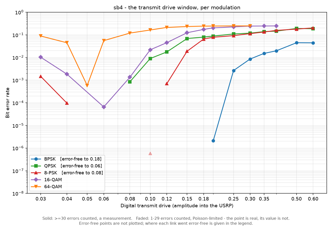
Measured on the sb4 pair, with the attenuator held at only 4 dB so the link has plenty of margin:
| amplitude | BPSK | QPSK | 8-PSK | 16-QAM | 64-QAM |
|---|---|---|---|---|---|
| 0.03 | 0 | 0 | 1.46e-3 | 1.03e-2 | 8.87e-2 |
| 0.04 | 0 | 0 | 9.67e-5 | 1.84e-3 | 4.48e-2 |
| 0.05 | – | – | – | – | 5.81e-4 ← best |
| 0.06 | 0 | 0 ← last clean | 0 | 6.58e-5 ← best | 5.55e-2 |
| 0.08 | 0 | 8.50e-4 | 0 ← last clean | 1.35e-3 | 1.20e-1 |
| 0.10 | 0 | 9.01e-3 | 5.76e-7 | 2.19e-2 | 1.64e-1 |
| 0.12 | 0 | 1.76e-2 | 6.98e-4 | 4.52e-2 | 2.13e-1 |
| 0.15 | 0 | 6.87e-2 | 1.89e-2 | 1.24e-1 | 2.34e-1 |
| 0.18 | 0 ← last clean | 7.96e-2 | 6.53e-2 | 1.74e-1 | 2.43e-1 |
| 0.20 | 2.12e-6 | 8.86e-2 | 7.83e-2 | 2.03e-1 | 2.45e-1 |
| 0.25 | 2.66e-3 | 1.09e-1 | 9.26e-2 | 2.26e-1 | 2.48e-1 |
| 0.30 | 8.57e-3 | 1.19e-1 | 1.13e-1 | 2.44e-1 | 2.49e-1 |
| 0.35 | 1.52e-2 | 1.39e-1 | 1.34e-1 | 2.46e-1 | no decode |
| 0.40 | 1.97e-2 | 1.46e-1 | 1.58e-1 | 2.48e-1 | no decode |
| 0.50 | 4.49e-2 | 1.91e-1 | 1.79e-1 | no decode | no decode |
| 0.60 | 4.45e-2 | 1.86e-1 | 2.03e-1 | no decode | no decode |
Three different things appear in that table and they are not interchangeable. A 0 is error-free — the sweep counted no errors at all, and the link is comfortable. A number is a measured BER. no decode is the opposite of error-free: the transmitter is so overdriven that frame sync fails and no packets arrive at all, so there is no BER to report. 64-QAM stops decoding above 0.30 and 16-QAM above 0.40, which is the far wall of the window.
Read across a row and the ordering is exactly what you would expect — at any drive, the denser the constellation the worse it does. Read down a column and you find the window: a floor, a wall, and for the two QAMs a clear minimum in between.
The QAM windows narrow with density, as theory says. The PSK family does not. 16-QAM peaks at 0.06 and 64-QAM at 0.05, and both stop decoding altogether well before BPSK is even troubled. But BPSK stays clean to 0.18 while 8-PSK stays clean to 0.08 and QPSK only to 0.06 — QPSK wants more back-off than the denser 8-PSK. That has now been reproduced on two different radios and at two different step resolutions. It is not a rounding artefact and it is not explained; it is recorded as measured.
Look at the 8-PSK column. It is the only one showing both walls: starved at 0.03, error-free between 0.06 and 0.10, distorted at 0.15 and above. That is the whole lesson of this part in one column — and it also shows that "a few percent BER with zero perfect packets" is not diagnostic on its own, because both ends of that column produce the signature from opposite causes. Only the direction of the trend tells you which way to move.
Run the probe with generous margin, or it measures the wrong thing. Lowering the amplitude lowers the received power too. On a link with little margin the low drive levels fail for lack of signal rather than from distortion, and the result is a window one point wide that says nothing about distortion at all. Our first attempt held the attenuator at 22 dB and produced exactly that.
The optimum is per-modulation and it is not ordered by constellation density: QPSK needs more back-off than 8-PSK on this hardware. Both sb4 (B205mini) and sb5 (B210) independently agree on QPSK 0.06, so it is reproducible, but we have no explanation we trust and report it as measured.
¶ Part 3 — Mechanism A: injected noise
Add a calibrated amount of AWGN at the receiver and hold everything else fixed. The noise is generated from a seed, so the same run reproduces byte-identical samples.
cosmos-run sdr/ofdm-ber-sb5.description.yml \
  -e '{"cosmos_parameters": {"sub": "bpsk", "amplitude": 0.15, "tx_gain": 89}}'
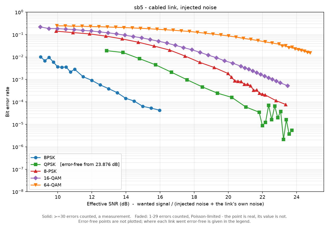
Over the air on grid, the same mechanism:
cosmos-run sdr/ofdm-ber-grid.description.yml \
  -e '{"cosmos_parameters": {"sub": "bpsk", "amplitude": 0.15, "tx_gain": 89}}'
¶ On grid, prefer the X310 pair
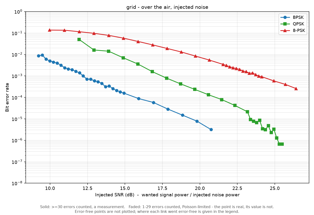
The command above uses the B210 pair at 2.4 GHz, which is what Figure 2 was measured on. It works, and it shares the band with the room's Wi-Fi.
The X310 pair at 2 GHz is the better link on every count — off the Wi-Fi band, 61.6 dB above the receiver's own noise floor against the B210 pair's 27.7, and error-free from 19 dB where the B210 pair bottoms out at 3.2 × 10⁻⁶:
cosmos-run sdr/ofdm-ber-grid-x310.description.yml \
  -e '{"cosmos_parameters": {"sub": "bpsk"}}'
Use it whenever you want the grid with margin to spare. Keep the B210 pair when you specifically want a link that is close to its limit — Figures 2 and 5 are more interesting precisely because that one is.
Do not simply retune the B210s to 2 GHz. That is the obvious move and it makes things worse, for a reason worth understanding: see the note above.
¶ Choosing what the noise is
The exact file format, and a dozen lines of Python that build AWGN or impulsive noise from scratch, are on Making a noise file.
The impairment does not have to be Gaussian, and this is the one thing neither an attenuator nor a transmit-power sweep can do — the noise is a recording, summed onto the received samples in the time domain, so it passes through frame sync and the channel estimator exactly as real interference would.
Three stock recordings are generated for you:
cosmos-run sdr/ofdm-ber-sb5.description.yml \
  -e '{"cosmos_parameters": {"noise_kind": "impulsive"}}'
noise_kind |
What it is |
|---|---|
awgn |
Flat Gaussian. The control — start here, because it is the curve theory predicts, and agreement with it is what earns trust in the stranger channels. |
coloured |
Gaussian with a shaped spectrum, so some subcarriers are hit harder than others. |
impulsive |
Gaussian background with 0.1 % of samples multiplied by 12 — the same total power concentrated into rare spikes, which is what a Gaussian-assuming receiver handles worst. |
Or bring your own. Point noise_file at a recording on the console and it is checked and shipped to the receiver for you:
cosmos-run sdr/ofdm-ber-sb5.description.yml \
  -e '{"cosmos_parameters": {"noise_file": "~/wifi-burst.sigmf-data"}}'
That is how you replay a real interferer: capture it once — a Wi-Fi burst, a microwave oven, a radar sweep — and run the identical recording against every modulation, which makes the comparison between modulations exact rather than merely fair.
- The format is raw interleaved complex64 — the
.sigmf-datahalf of a SigMFcf32_lepair, never the.sigmf-metahalf. - The level does not matter. The sweep measures the recording's own RMS and scales it to hit each requested SNR, so a capture taken at any gain gives the same curve.
- A recording shorter than the capture is replayed to cover it. Aim for more than eight sweep strides (about 500 k samples) so consecutive points are independent draws rather than the same realisation at different amplitudes — the run warns you if it is shorter.
noise_file_on_nodenames a file already on the receiver instead, for a recording too large to push on every run. Set at most one of the two.
The path is validated on the console before any hardware is touched, so a typo costs about eight seconds rather than a node bring-up.
¶ The link's own noise counts too — the axis already includes it
Injected noise does not replace the noise the receiver already has, it adds to it. So the ratio the receiver actually experiences is
effective SNR = wanted signal / (injected noise + the link's own noise)
and it is always worse than the number you asked for. As the requested SNR climbs the injected term shrinks until the link's own noise dominates, at which point the effective SNR stops rising: it can never exceed the link's margin over its own noise floor. Ask for 26 dB on a link with 17 dB of margin and the injected noise is far below the noise already present — the point measures the link, returns a plausible number, and the curve flattens.
That flat part looks exactly like a modulation-dependent error floor. It is not. Three curves in this laboratory were wrong for that reason before it was corrected: the QPSK curve on sb5 appeared to bottom out at 9e-4 until the transmit gain was raised, after which it reached 2.1e-6 and went error-free.
So each run measures the floor before it starts — with the transmitter off — and derives the effective SNR from it. Both numbers are printed, and it is the effective one the figures are plotted against:
received RMS 0.020742, floor 0.00027738 -> signal RMS 0.020741 (37.5 dB above floor)
asked    eff SNR  noise       bytes      packets  errors    BER          perfect
If asked and eff SNR diverge by more than a decibel or two at the top of your range, raise the transmit gain. Backing the drive off for a denser constellation costs margin, so drive and gain have to be set together.
And even the effective SNR is an upper bound. The floor is measured with the transmitter switched off, so it captures thermal noise, the receiver's own noise figure and whatever ambient interference is in the band — but nothing the transmitter contributes. Transmit distortion, quadrature imbalance, oscillator phase noise and the like appear only while transmitting, and no floor measurement will ever see them.
That gap can be large. On the sb1 FR3 chain the transmit and receive hardware together impose an error-vector floor near 15 dB effective SNR — measured by decomposing the error vector directly — while the received signal sits 29 dB above the noise floor. A sweep on that chain that trusted the floor alone would believe it had 29 dB to play with and would report a modulation limit at the point where the hardware, not the modulation, ran out.
The practical rule: the effective-SNR axis is honest about noise, and silent about distortion. When a curve flattens and the two SNR columns still agree, distortion is the next thing to look at — start with the drive window in Part 2.
¶ Part 4 — Mechanism B: path attenuation
Only sb4 has the programmable matrix, and it is the cleanest of the three: the signal genuinely arrives weaker, so thermal noise sets the floor exactly as distance would. There is no SNR ceiling — nothing is being added, so nothing can fall below the link's own noise.
cosmos-run sdr/ofdm-ber-sb4.description.yml \
  -e '{"cosmos_parameters": {"sub": "bpsk", "amplitude": 0.15}}'
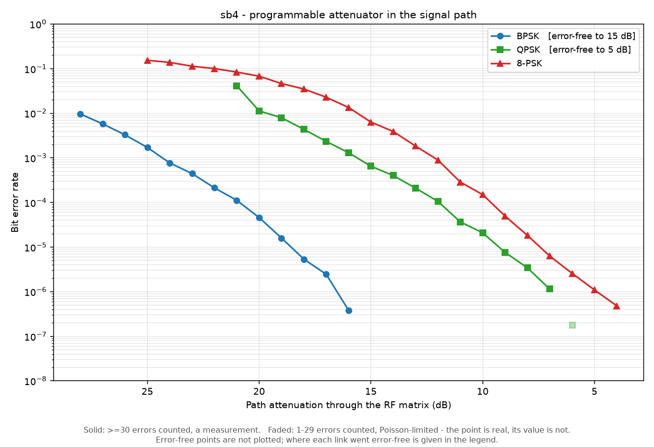
The matrix service takes attenuation as a whole number of decibels, so 1 dB is the finest step available here — the noise and transmit-power sweeps can be finer.
Reading Figure 3. The decode cliffs are BPSK 28 dB, QPSK 21 dB, 8-PSK 25 dB — so 8-PSK survives more attenuation than QPSK, which is the wrong way round for constellation density. It is not a modulation result: each curve runs at its own optimum drive, and 8-PSK's 0.10 is about 4.4 dB hotter than QPSK's 0.06. Add that back and QPSK's cliff lands near 26 dB, in the expected order. The curves are deliberately not power-normalised, because the drive level is part of what each modulation needs.
¶ Part 5 — Mechanism C: transmit power, and why not to use it
Change nothing but the transmit gain.
cosmos-run sdr/ofdm-ber-grid-txpower.description.yml
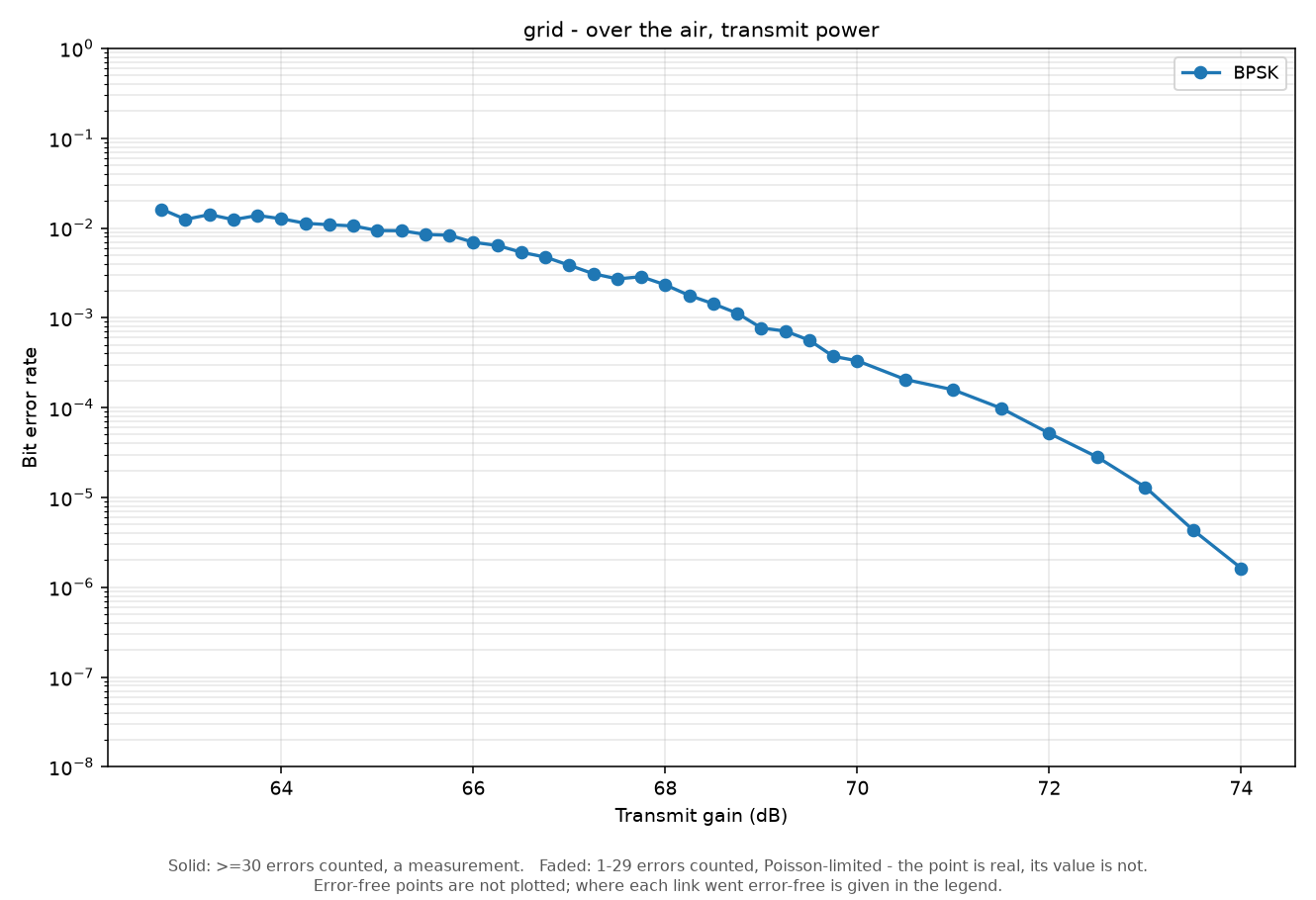
It works, and it needs no extra hardware — but it is the worst of the three as an SNR axis, for four reasons this curve shows directly:
- The steps are quantised. A B210 resolves 0.25 dB on transmit (0–89.75 dB) and 1.0 dB on receive, so this resolution exists only on the transmit side.
- Gain is not SNR. Delivered power goes non-linear as the chain compresses, so equal gain steps are not equal SNR steps.
- The tail is unaffordable. At 66 dB the sweep counted 500 errors in 10 s; at 74 dB it found 63 in 120 s. Reaching 1e-7 would cost roughly an hour per point — 500 errors at 1e-7 is 5×10⁹ bits, which at 1 MSps is about 1.7 hours.
- It moves the drive. Raising gain changes where the transmitter sits relative to compression, which is the very thing Part 2 asked you to pin down.
Use it to find an operating point, not to measure a waterfall.
When it is nonetheless the right choice. Everything above assumes you have an alternative. The FR3 tutorial uses transmit power for all five modulations, because on that link the other two are unavailable: there is no attenuator matrix in the path, and injected noise runs into the ceiling described in Part 3 long before it reaches the dense constellations. Pick the mechanism by what the link offers, not by a ranking — and when you do use transmit power, re-probe the drive window afterwards, because you have moved it.
¶ Verification
Your curves will not match ours exactly — a different pair of nodes, a different day and a different antenna position all move them — but these are the shapes and the landmarks to check.
BPSK, all three mechanisms:
| Mechanism | Curve spans | Error-free at |
|---|---|---|
| A, cabled (sb5) | 8.4e-3 → 3.7e-7 | 23 dB SNR |
| A, over the air (grid) | 8.6e-3 → 3.2e-6 | — (range stopped at 21 dB) |
| B, attenuator (sb4) | 4.1e-2 → 3.8e-7 | ≤15 dB attenuation |
| C, transmit power (grid) | 1.6e-2 → 1.6e-6 | — (stopped at 1e-6) |
Checks that matter more than the numbers:
- The curve is monotonic. A waterfall that flattens or wanders is telling you something is wrong — most likely that you have run past the link's margin, or that the transmitter is overdriven.
- Perfect-packet count rises with SNR. If BER is a few percent and perfect packets are zero across the whole sweep, you are outside the drive window. Go back to Part 2.
- The
askedandeff SNRcolumns agree to within a decibel over most of your range. - Nothing decodes below about 9 dB. Every mechanism shows this wall. Measured: 8.74 dB on the cabled sb5 link, 9.23 dB on the over-the-air grid link — half a decibel apart on completely different paths, different hardware and different margins. That makes it a property of the receiver: below it the OFDM frame detector stops finding headers, no payload is emitted, and there is no BER to compute. It is an absence, not a floor.
On reading a waterfall honestly:
- A point with zero errors is not a BER. It is an upper bound of 1/bits. Plotting it on a log axis means inventing a value, so these figures do not plot it; the legend states where each link went error-free instead.
- A BER estimate's precision depends on the number of errors counted, not the number of bits: the relative scatter is roughly 1/√(errors). Thirty errors is about ±18 %; five hundred is about ±4.5 %. That is why each point here captures until it has accumulated a target error count rather than for a fixed time — a fixed dwell over-measures the noisy end and under-measures the tail.
¶ Cleanup
Stop any transmitter you started by hand, then release the nodes:
ssh root@node1-1 'systemctl stop ofdmtx.service' 2>/dev/null
omf tell -a offh -t node1-1,node1-2
The automated path stops its transmitter in an always: block, so it is stopped even when a run fails — but check anyway if you interrupted one:
ssh root@node1-1 'systemctl is-active ofdmtx.service cosmos-fr3-ofdm-tx.service'
On sb4, the attenuators are left where the sweep put them. That is deliberate — the next experimenter should find a known state rather than one you invented — but note it if you are sharing the sandbox.
¶ Troubleshooting
| Symptom | Likely cause | Fix |
|---|---|---|
| A few percent BER and zero perfect packets at every setting | Transmitter overdriven, or starved | Run Part 2. Both causes give this signature; the trend direction distinguishes them |
| Curve flattens at some BER and will not go lower | Sweep is asking for more SNR than the link's margin over thermal | Raise the transmit gain; compare the asked and eff SNR columns |
| No decode at all, at any setting | Receiver never started | Check the receiver's own stderr. A missing noise file kills it at construction with RuntimeError: can't open file |
Permission denied sshing to a node |
Node is still in the PXE stage image, not your image | omf tell offh then on; verify with cat /.omf-image-name |
Wrong SDR selected on grid |
Node can reach ~20 networked X310s | Pin the local radio with --dev-args="type=b200" |
RF matrix returns undefined method '[]' for nil |
switch and port passed the wrong way round |
switch is the switch number, port the position (1 = WiFi, 2 = SDR) |
| Link is tens of dB weaker than expected | Measured before the B210 settled | Wait ~12 s after starting the transmitter |
omf load said success but the node runs the wrong image |
Known omf load false success |
Verify each node with cat /.omf-image-name |
¶ References
- SDR hardware on COSMOS
- OMF commands
- GNU Radio OFDM examples
- Schmidl, T.M. and Cox, D.C., "Robust frequency and timing synchronization for OFDM", IEEE Trans. Communications, 1997 — the synchroniser this receiver uses.
Author(s): COSMOS · Last verified: 2026-08-01 · Tested image/release: baseline-sdr.ndz (UHD 4.9, GNU Radio 3.10.12) · Tags: sdr, gnuradio, ofdm, ber, modulation